AI_ML_DL’s diary

人工知能、機械学習、ディープラーニングの日記

ARC コンペのコードに学ぶ

KaggleのARCコンペ第3位、Ilia Larchwnko氏の手法に学ぶ


目的は、Domein Specific Languageにより、課題を解くことができるようにすること。


ARCコンペの7位以内で、かつ、GitHubで公開しているものの中から選んだ。

Ilia氏は、2名で参加していて、最終結果は0.813(19/104)であるが、GitHubで公開しているのは、Ilia氏単独のもので、単独での正解数は正確にはわからない。

Kaggleのコンペサイトに公開されているnotebooksは、19/104の好成績を得ているものであるが、複数のコードが混ざっている。


GitHubに公開されている、Ilia氏単独開発のコードは、全体の構成がわかりやすい。train dataでの正解は138/400、evaluation dataでの正解は96/400とのことである。 


ソースコードは、大きくは、predictors(約4500行)とpreprocessing(約1300行)とfunctions(約160行)に分かれている。

predictorsでは、functionsから、

1.

combine_two_lists(list1, list2):

2.

filter_list_of_dicts(list1, list2): 

      """ returns the intersection of two lists of dicts """

3.

find_mosaic_block(image, params):

      """ predicts 1 output image given input image and prediction params """

4.

intersect_two_lists(list1, list2):

      """ intersects two lists of np.arrays """

5.

reconstruct_mosaic_from_block(block, params, original_image=None):

6.

swap_two_colors(image):

      """ swaps two colors """

preprocessingからは、

1.

find_color_boundaries(array, color):

      """ looks for the boundaries of any color and returns them """

2.

find_glid(image, frame=False, possible_colors=None):

      """ looks for the grid in image and returns color and size """

3.

get_color(color_dict, colors):

      """ retrive the absolute number corresponding a color set by color_dict """

4.

get_color_max(image, color):

      """ return the part of image inside the color boundaries """

5.

get_dict_hash(d):

6.

get_grid(image, grid_size, cell, frame=False):

      """ returns the particular cell form the image with grid """

7.

get_mask_from_block_params(image, params, block_cashe=None, mask_cashe=None, color_scheme=None)

8.

get_predict(image, transform, block_cash=None, color_scheme=None):

      """ applies the list of transforms to the image """

9.

preprosess_sample(sample, param=None, color_param=None, process_whole_ds=False):

      """ make the whole preprocessing for particular sample """

が呼び出され、

predictorsには、以下のクラスがある。

1. Predictor

2.

Puzzle(Predictor):

      """ Stack different blocks together to get the output """

3.

PuzzlePixel(puzzle):

      """ very similar to puzzle but applicable only to pixel_level blocks """

4.

Fill(predictor):

      """ applies different rules using 3x3 masks """

5.

Fill3Colors(Predictor):

      """ same as Fill but iterates over 3 colors """ 

6.

FillWithMask(Predictor):

      """ applies rules based on masks extracted from images """

7.

FillPatternFound(Predictor):

      """ applies rules based on masks extracted from images """

8.

ConnectDot(Predictor):

      """ connect dot of same color, on one line """

9.

ConnectDotAllColors(Predictor):

      """ connect dot of same color, on one line """

10

FillLines(Predictor):

      """ fill the whole horizontal and/or vertical lines of one color """

11.

ReconstructMosaic(Predictor)

      """ reconstruct mosaic """

12.

ReconstructMosaicRR(Predictor):

      """ reconstruct mosaic using rotations and reflections """

13.

ReconstructMosaicExtract(ReconstructMosaic):

      """ returns the reconstructed part of the mosaic """

14.

ReconstructMosaicRRExtract(ReconstructMosaicRR):

      """ returns the reconstructed part of the rotate/reflect mosaic """

15.

Pattern(Predictor)

      """ applies pattern to every pixel with particular color """

16.

PatternFromBlocks(Pattern):

      """ applies pattern extracted form some block to every pixel with particular color """

17.

Gravity(Predictor):

      """ move non_background pixels toward something """

18.

GravityBlocks(Predictor):

      """ move non_background objects toward something """

19.

GravityBlocksToColors(GravityBlocks):

      """ move non_background objects toward color """

20.

GravityToColor

21. EliminateColor

22. EliminateDuplicate

23. ReplaceColumn

24. CellToColumn

25. PutBlochIntoHole

26. PutBlockOnPixel

27. EliminateBlock

28. InsideBlock

29. MaskToBlock

30. Colors

31. ExtendTargets

32. ImageSlicer

33. MaskToBlockParallel

34. RotateAndCopyBlock


わかりやすい課題を1つ選んで、詳細を見ていこう。 


まず最初に、入力として与えられたもの(イメージ、図柄、グリッドパターン)の、colorと、blockと、maskを、JSON-like objectで表現する。

JSONの文法は、こんな感じ。

{ "name": "Suzuki", "age": 22}


それぞれ、以下のように説明されている。

しかし、これだけ見ても、なかなか、理解できない。

実際のパターンと見比べたり、preprocessing.pyのコードを見て学んでいくしかない。

この作業は、ARCの本質的な部分でもあるので、じっくり検討しよう。 

2.1.1 Colors

I use a few ways to represent colors; below are some of them:

  • Absolute values. Each color is described as a number from 0 to 9. Representation: {"type”: "abs”, "k”: 0}

  • あらかじめ決められている数字と色の対応関係:0:black,  1:blue,  2:red,  3:green,  4:yellow,  5:grey,  6:magenda,  7:orange,  8:sky,  9:brown
  • The numerical order of color in the list of all colors presented in the input image sorted (ascending or descending) by the number of pixels with these colors. Representation: {"type”: "min”, "k”: 0}{"type”: "max”, "k”: 0}

  • 色の並び、0(黒)を最大とみなすか、最小とみなすか。どういう使い方をするのだろうか。
  • The color of the grid if there is one on the input image. Representation: {"type”: "grid_color”}

  • 単色(出力に単色はあるが、入力で単色というのはあっただろうか)。それとも、黒地に単色パターンという意味だろうか。
  • The unique color in one of the image parts (top, bottom, left, or right part; corners, and so on). Representation: {"type": "unique", "side": "right"}{"type": "unique", "side": "tl"}{"type": "unique", "side": "any"}

  • 上下左右隅のどこかの部分の色だけが異なっている。"tl"は、top+leftのことだろうか?
  • No background color for cases where every input has only two colors and 0 is one of them for every image. Representation: {"type": "non_zero"}

  • 入力グリッドが2色からなっている場合に、通常は、0:黒をバックグラウンドとして扱うが、黒が他の色と同じように扱われている場合には、"non_zero"と識別するということか。

Etc.

2.1.2 Blocks

Block is a 10-color image somehow derived from the input image.

Each block is represented as a list of dicts; each dict describes some transformation of an image.

One should apply all these transformations to the input image in the order they are presented in the list to get the block.

Below are some examples.

The first order blocks (generated directly from the original image):

  • The image itself. Representation: [{"type": "original"}]

  • One of the halves of the original image. Representation: [{"type": "half", "side": "t"}][{"type": "half", "side": "b"}][{"type": "half", "side": "long1"}]

  • 上半分、下半分、"long1":意味不明
  • "t" : top,  "b" : bottom
  • The largest connected block excluding the background. Representation: [{"type": "max_block", "full": 0}]

  • バックグラウンド以外で、もっとも大きなブロックに着目する、ということか。"full": 0は、バックグラウンドが黒(0)ということか?
  • The smallest possible rectangle that covers all pixels of a particular color. Representation: [{"type": "color_max", "color": color_dict}] color_dict – means here can be any abstract representation of color, described in 2.1.1.

  • 特定の色で最小サイズの矩形ブロックのことか?"color_max"の意味が不明
  • Grid cell. Representation: [{"type": "grid", "grid_size": [4,4],"cell": [3, 1],"frame": True}]

  • グリッドが全体で、セルは部分を指しているのか?
  • The pixel with particular coordinates. Representation: [{"type": "pixel", "i": 1, "j": 4}]

  • particular coordinateとi,jの関係が不明

Etc.

The second-order blocks – generated by applying some additional transformations to the other blocks:

  • Rotation. Representation: [source_block ,{"type": "rotation", "k": 2}] source_block means that there can be one or several dictionaries, used to generate some source block from the original input image, then the rotation is applied to this source block

  • 回転、"k"は単位操作の繰り返し回数か?
  • Transposing. Representation: [source_block ,{"type": "transpose"}]

  • "transpose" : 行と列を入れ替える
  • Edge cutting. Representation: [source_block ,{"type": "cut_edge", "l": 0, "r": 1, "t": 1, "b": 0}] In this example, we cut off 1 pixel from the left and one pixel from the top of the image.

  • 端部のカット:数字がピクセル数だとすれば、rightとtopから1ピクセルカットするということになる。説明が間違っているのか?
  • Resizing image with some scale factor. Representation: [source_block , {"type": "resize", "scale": 2}][source_block , {"type": "resize", "scale": 1/3}]

  • 2倍、3分の1倍
  • Resizing image to some fixed shape. Representation: [source_block , {"type": "resize_to", "size_x": 3, "size_y": 3}]

  • x方向に3倍、y方向にも3倍ということか?
  • Swapping some colors. Representation: [source_block , {"type": "color_swap", "color_1": color_dict_1, "color_2": color_dict_2}]

  • 色の交換

Etc.

  • There is also one special type of blocks - 
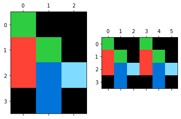
[{"type": "target", "k": I}]. It is used when for the solving ot the task we need to use the block not presented on any of the input images but presented on all target images in the train examples. Please, find the example below.
  • 次の図のように、入力画像に含まれず、出力画像(target)にのみ含まれるブロック構造を指す。

train1

2.1.3 Masks

Masks are binary images somehow derived from original images. Each mask is represented as a nested dict.

  • Initial mask literally: block == color. Representation: {"operation": "none", "params": {"block": bloc_list,"color": color_dict}} bloc_list here is a list of transforms used to get the block for the mask generation

  • Logical operations over different masks Representation: {"operation": "not", "params": mask_dict}, {"operation": "and", "params": {"mask1": mask_dict 1, "mask2": mask_dict 2}}, {"operation": "or", "params": {"mask1": mask_dict 1, "mask2": mask_dict 2}}, {"operation": "xor", "params": {"mask1": mask_dict 1, "mask2": mask_dict 2}}

  • Mask with the original image's size, representing the smallest possible rectangle covering all pixels of a particular color. Representation: {"operation": "coverage", "params": {"color": color_dict}}

  • Mask with the original image's size, representing the largest or smallest connected block excluding the background. Representation: {"operation": "max_block"}

オリジナルイメージサイズのマスクの例

オリジナルイメージを4x4に拡大した後に、オリジナルイメージでマスクしている!

train1

以下の2組もマスクの例

f:id:AI_ML_DL:20200605120419p:plain

f:id:AI_ML_DL:20200605120609p:plain

You can find more information about existing abstractions and the code to generate them in preprocessing.py.


2.2 Predictors

I have created 32 different classes to solve different types of abstract task using the abstractions described earlier.

All of them inherit from Predictor class.

The general logic of every predictor is described in the pseudo-code below (also, it can be different some classes).


for n, (input_image, output_image) in enumerate(sample['train']):

      list_of_solutions = [ ]

      for possible_solution in all_possible_solutions:

            if apply_solution(input_image, possible_solution) == output_image:

                  list_of_solutions.append(possible_solution)

      if n == 0:

            final_list_of_solutions = list_of_solutions

      else:

            final_list_of _solutions = intersection(list_of_solutions, final_list_of _solutions)


      if len(final_list_of_solutions == 0

            return None


answers = [ ]

for test_input_image in sample['test']:

      answers.append([ ])

      for solution in final_list_of_solutions:

            answers[-1].append(apply_solution(test_input_image, solution))


return answers


The examples of some predictors and the results are below.

・Puzzle - generates the output image by concatenating blocks generated from the input image

train42.png

見た目は非常に簡単なのだが、プログラムは130行くらいある。

まずは、写経

# puzzle like predictors

class Puzzle(Predictor):

      """ Stack different blocks together to get the output """

      def __init__(self, params=None, preprocess_params=None):

            super( ).__init__(params, preprocess_params)

            self.intersection = params["intersection"]


      def initiate_factors(self, target_image):

            t_n, t_m = target_image.shape

            factors = [ ]

            grid_color_list = [ ]

            if self.intersection < 0:

                  grid_color, grid_size, frame = find_grid(target_image)

                  if grid_color < 0:

                        return factors, [ ]

                  factors = [glid_size]

                  grid_color_list = self.sample["train"][0]["colors"][glid_color]

                  self.frame = frame

            else:

                  for i in range(1, t_n, + 1):

                        for j in range(1, t_m + 1):

                            if (t_n - self.intersection) % 1 == 0 and (t_m - self.intersection) % j == 0:

                                factors.append([i, j])

            return factors, grid_color_list


*ここで、preprocessingのfind_grid( )を見ておこう。


def find_grid(image, frame=False, possible_colors=None):

      """ Looks for the grid in image and returns color and size """

      grid_color = -1

      size = [1, 1]

      if possible_colors is None:

            possible_colors = list(range(10))

      for color in possible_colors:

            for i in range(size[0] +1, image.shape[0] // 2 + 1):

                  if (image.shape[0] +1) % i == 0:

                        step = (image.shape[0] +1) // i

                        if (image[(step - 1) : : step] == color).all( ):

                              size[0] = i

                              grid_color = color

            for i in range(size[1] +1, image.shape[1] // 2 + 1):

                  if (image.shape[1] +1) % i == 0:

                        step = (image.shape[1] +1) // i

                        if (image[(step - 1) : : step] == color).all( ):

                              size[1] = i

                              grid_color = color


preprocessing.pyのコードの簡単なものから眺めていこう。


1.

def get_rotation(image, k):

      return 0, np.rot90(image, k)

kは整数で、回転角は、90 * kで、反時計回り。


2.

def get_transpose(image):

      return 0, np.transpose(image)

行と列の入れ替え(転置)


3.

def get_roll(image, shift, axis)

      return 0, np.roll(image, shift=shift, axis=axis)


*またまた、途中で放り出すことになってしまった。

*ARCに興味がなくなった。

*知能テストを、ヒトが解くように解くことができるプログラムを開発するという目的において、重要なことは、例題から解き方を学ぶこと。

*ARCは、どれも、例題が3つくらいある。複数の例題があってこそ、出力が一意に決まるものもあるが、1つの例題だけで済ませた方が楽しものも多く、それで出力が一意に決まるものを見つける方が楽しい。

*あえて言えば、例題はすべて1つにして、複数の正解があってもいいのではないだろうか。

*あとは、やはり、1つしかない例題から、変換方法を見つけ出すことを考えるようなプログラムを作ってみたいと思うので、そちらをやってみる。


おわり 


f:id:AI_ML_DL:20200602101441p:plain

style=146 iteration=1

f:id:AI_ML_DL:20200602101548p:plain

style=146 iteration=20

f:id:AI_ML_DL:20200602101641p:plain

style=146 iteration=500


Chapter 19 Training and Deploying TensorFlow Models at Scale

Chapter 19  Training and Deploying TensorFlow Models at Scale

Hands-On Machine Learning with Scikit-Learn, Keras & Tensorflow 2nd Edition by A. Geron


Chapter 2は、KaggleのTitanicと並行して勉強していたので、何をどこまで学んだか忘れてしまったが、章のタイトルが"End-to-End Machine Learning Project"となっていて、最後の方に、"Lauch, Monitor, and Maintain Your System"という節があって、開発した機械学習モデルを市場に出して運用するところまで説明されていたのが強く印象に残っている。

プログラム開発は、モノづくりであって、市場に出してナンボ。

誰が、どこで、どのように使うのかを想定しておかないと、収集したデータも、開発したプログラムも、使われることなく埋もれてしまうことになりかねない。

研究開発して、論文発表して終わりということなら、関係ないかもしれない。

それでも、この分野の今後の発展を考えるならば、常に変化している最先端の開発環境を使えるようにしておくことも含めて、勉強しておこう。

ということで、まず、第2章の該当部分を復習することから始めよう。


Chapter 2: End-to-End Machine Learning Project

Lauch, Monitor, and Maintain Your System

Perfect, you got approval to launch!

You now need to get your solution ready for production (e.g., polich the code, write documantation and test, and so on).

Then you can deploy your model to your production environment.

One way to do this is to save the trained Scikit-Learn model (e.g., using joblib), including the full preprocessing and prediction pipeline, then load this trained model within your production environment and use it to make predictions by calling its predict( ) method.

For example, perhaps the model will be used within a website:

the user will type in some data about a new distinct and click the Estimate Price button.

This will send a query containing the data to the web server, which will forward it to your web application, and finally your code will simply call the model's predict( ) method (you want to load the model upon server startup, rather than every time the model is used).

Alternatively, you can wrap the model within a dedicated web service that your web application can query through a REST API.

REST API: In a nutshell, a REST (or RESTful) API is an HTTP-based API that follows some conventions, such as using standard HTTP verbs to read, update, or delete resources (GET, POST, PUT, and DELETE) and using JSON for the inputs and outputs.

This makes it easier to upgrade your model to new versions without interrupting the main application.

It also simplifies scaling, since you can start as many web services as needed and load-balance the requests coming from your web application across these web services.

Moreover, it allows your web application to use any language, not just Python.


Anothe popular strategy is to deploy your model on the cloud, for eample on Google Cloud AI Platform (formerly known as Google Cloud ML Engine):

just save your model using joblib and upload it to Google Cloud Storage (GCS), then head over to Google Cloud AI Platform and create a new model version, pointing it to the GCS file.

That's it!

This gives you a simple web service that takes care of load balancing and scaling for you.

It takes JSON requests containing the input data (e.g., of a district) and return JSON responses containing the predictions.

You can then use this web service in your website (or whatever production environment you are using).

As we will see in Chapter 19, deploying TensorFlow models on AI Platform is not much different from deploying Scikit-Learn models.


But deployment is not the end of the story.

You also need to write monitoring code to check your system's live performance at regular intervals and trigger alerts when it drops.

This could be a steep drop, likely due to a broken component in your infrastructure, but be aware that it could also be a gentle decay that could easily go unnoticed for a long time.

This is quite common because models tend to "rot" over time:

indeed, the world changes, so if the model was trained with last year's data, it may not be adapted to today's data.


Even a model trained to classify pictures of cats and dogs may need to be retrained regularly, not because cameras keep changing, along with image formats, sharpness, brightness, and size ratios.

Moreover, people may love different breeds next year, or they may decide to dress their pets with tiny hats - Who knows?


So you need to monitor your model's live performance.

But howdo you that?

Well, it depends.

In some cases the model's performance can be infered from downstream metrics.

Fore example, if your model is part of a recommender system and it suggests products that the users may be interested in, then it's easy to monitor the number of recommended products sold each day.

If  this number drops (compared to nonrecommended products), then the prime suspect is the model.

This may be because the data pipeline is broken, or perhaps the model needs to be retrained on fresh data (as we will discuss shortly).


However, its not always possible to determine the model's performance without any human analysis.

For example, suppose you trained an image classification model (see Chapter 3) to detect several product defects on a production line.

How can you get an alert if the model's performance drops, before thousands of defective products get shipped to your cliants?

One solution is to send to human raters a sample of all the pictures that the model classified (especially pictures that the model wasn't so sure about).

Depending on the task, the raters may need to be experts, or they could be nonspecialists, such as workers on a crowdsourcing platform (e.g., Amazon Mechanical Turk).

In some applications they could even be the users themselves, responding for example via surveys or repurposed captchas.


Either way, you need to put in place a monitoring system (with or without human raters to evaluate the live model), as well as all the relevant processes to define what to do in case of failures and how to prepare for them.

Unfortunately, this can be a lot of work.

In fact, it is often much more work than building and training a model.


そりゃあ、遊び用のモデルと違って、生産工場で使うモデルは、根本的に違った設計になるのは当然である。

初期性能の維持は当然であり、欠陥の見逃しなど許されるはずがない。

最低でも、不良品の検出と良品の検出はパラレルで走らさないといけない。

良品と不良品の検知の経験を、モデルに対して定期的にフィードバックして、モデルの性能を向上させていくべきものでしょう。

ハードウエアの向上にも対応しないといけないし、それによる性能アップも必要。

複数のモデルを多重に走らせることが必要だろうな。

性能だけなら、凝ったディープラーニングモデルが高い性能を示すかもしれないが、そのDNNモデルにしても、簡単なものから複雑なものまでパラレルに走らせばいいし、予測能力の数値は低くても、安定して動作する機械学習モデルも並行して走らせておけばいいだろうし、・・・。

ランダムにサンプリングした高精度画像をオフラインで定期的に、あるいは、徹底的に検査・精査することも必要だろうし・・・。

画像も、可視だけでなく、赤外とか紫外とか、さらに、レーザー照射して干渉光を利用分光するとか、高速ラマン分光を使うとか、X線や電子線を照射して特性X線を検出するとか、・・・。


If the data keeps evolving, you will need to update your datasets and retrain your model regularly.

You should probably automate the whole process as much as possible.

Here are a few things you can automate:

・Collect fresh data regularly and label it (e.g., using human raters).

・Write a script to train the model and fine-tune the hyperparameters automatically.

   This script could run automatically, fore example every day or every week, depending       on your needs.

・Write another script that will evaluate both the new model and the previous model on     the updated test set, and deploy the model to production if the performance has not       decreased (if it did, make sure you investigate why).


You should also make sure you evaluate the model's input data quality.

Sometimes performance will degrade slightly because of a poor-quality signal (e.g., a malfunctioning sensor sending random values, or another team's output becoming stale), but it may take a while before your system's performance degrades enough to trigger an alart.

If you monitor your model's inputs, you may catch this earlier.

For example, you could trigger an alert if more and more inputs are missing a feature, or if its mean or standard deviation drifts too far from the training set, or a categorical feature starts containing new categories.


Finally, make sure you keep backups of every model you create and have the process and tools in place to roll back to a previous model quickly, in case the new model starts failing badly for some reason.

Having backups also makes it possible to easily compare new models with previous ones.

Similarly, you should keep backups of every version of your datasets so that you can roll back to a previous dataset if the new one ever gets corrupted (e.g., if the fresh data that gets added to it turns out to be full of outliers).

Having backups of your datasets also allows you to evaluate any model against any previous dataset.


You may want to create several subsets of the test set in order to evaluate how well your model performs on specific parts of the data.

For example, you may want to have a subset containing only the most recent data, or a test set for specific kinds of inputs (e.g., districts located inland versus districts located near the ocean).

This will give you a deeper understanding of your model's strengths and weaknesses.


As you can see, Machine Learning involves quite a lot of infrastructure, so don't be surprized if your first ML project takes a lot of effort and time to build and deploy to production.

Fortunately, once all the infrastructure is in place, going from idea to production will be much faster.


Chapter 19  Training and Deploying TensorFlow Models at Scale


A great solution to scale up your service, as we will see in this chapter, is to use TF Serving, either on your own hardware infrastructure or via a cloud service such as Google Cloud AI Platform.

It will take care of efficiently serving your model, handle graceful model transitions, and more.

If you use the cloud platform, you will also get many extra features, such as powerful monitoring tools.


In this chapter we will look at how to deploy models, first to  


f:id:AI_ML_DL:20200520094423p:plain

style=140 iteration=1


f:id:AI_ML_DL:20200520094510p:plain

style=140 iteration=20


f:id:AI_ML_DL:20200520094550p:plain

style=140 iteration=500


Chapter 18 Reinforcement Learning

Chapter 18  Reinforcement Learning

Hands-On Machine Learning with Scikit-Learn, Keras & Tensorflow 2nd Edition by A. Geron


Reinforcement Learning (RL) is one of the most exciting fields of Machine Learning today, and  also one of the oldeat.

It has been around since the 1950s, producing many interesting applications over the years, particularly in games (e.g., TD-Gammon, a Backgammon-playing program) and in machine control, but seldom making the headline news.

But a revolution took place in 2013, when researchers from a British startup called DeepMind demonstrated a system that could learn to play just about any Atari game from scratch (https://homl.info/dqn), eventually outperforming humans (https://homl.info/dqn2) in most of them, using only raw pixels as imputs and without any prior knowledge of the rules of the games.

This was the first of a series of amazing feats, culminating in March 2016 with the victory of their system AlphaGo against Lee Sedol, a legendary professional player of the game of Go, and in May 2017 against Ke Jie, the world champion.

No program had ever come close to beating a master of this game, let alone the world champion.

Today the whole field of RL is boiling with new ideas, with a wide range of applications.

DeepMind was bought by Google for over $500 million in 2014.


So how did DeepMind achieve all this?

With hindsight it seems rather simple: they applied the power of Deep Learning to the field of Reinforcement Learning, and it worked beyond their wildest dreams.

In this chapter we will first explain what Reinforcement Learning is and what it's good at, then present two of the most important techniques in Deep Reinforcement Learning: policy gradients and deep Q-networks (DQNs), including a discussion of Markov decision processes (MDPs).

We will use these techniques to train models to balance a pole on a moving cart; then I'll introduce th TF-Agents library, which uses state-of-the-art algorithms that greatly simplify building powerful RL systems, and we will use the librsry to train an agent to play Breakout, the famous Atari game.

I'll close the chapter by taking a look at some of the latest advances in the field.


Learning to Optimize Rewards

In Reinforcement Learning, a software agent makes observations and takes actions within an environment, and in return it receives rewards.

Its objective is to learn to act in a way that will maximize its expected rewards over time.

If you don't mind a bit of anthropomorphism, you can think of positive rewards as pleasure, and negative rewards as pain ( the term "reward" is a bit misleading in this case).

In short, the agent acts in the environment and learns by trial and error to maximize its pleasure and minimize its pain.

This is quite a broad setting, which can apply to a wide variety of tasks.

Here are a few examples (see Figure 18-1):

a.  The agent can be the program controlling a robot.

     In this case, the environment is the real world, the agent observes the environment           through a set of sensors such as cameras and touch sensors, and its actions consist of       sending signals to active motors.    

     It may be programmed to get positive rewards whenever it approaches the target             destination, and negative rewards whenever it wastes time or goes in the wrong               direction.

b.  The agent can be the program controlling Ms. Pac-Man.

     In this case, the environment is a simulation of the Atari game, the actions are the             nine possible joystick positions (upper left, down, center, and so on), the observations       are screenshots, and the rewards are just the game points.

c.  Similarly, the agent can be the program playing a board game such as Go.

d.  The agent does not have to control a physically (or virtually) moving thing.

     For example, it can be a smart thermostat, getting positive rewards whenever it is             close to the target temperature and saves energy, and negative rewarda when                   humans need to tweak the temperature, so the agent must learn to anticipate human       needs.

e.  The agent can observe stock market prices and decide how much to buy or sell every       second.  

     Rewards are obviously the monetary gains and losses.


Note that there may not be any positive rewards at all; for example, the agent may move around in a maze, getting a negative reward at every time step, so it had better find the exit as quickly as possible!

There are many other examples of tasks to which Reinforcement Learning is well suited, such as self-driving cars, recommender systems, placing ads on a web page, or controlling where an image classification system should focus its attention.


Policy Search

The algorithm a software agent uses to determine its actions is called its policy.

The policy couuld be a neural network taking obsevations as inputs and outputting tha action to take (see Figure 18-2).


The policy can be any algorithm you can think of, and it does not have to be deterministic.

In fact, in some cases it does not even have to observe the environment!

For example, consider a robotic vacuum cleaner whose reward is the amount of dust it picks up in 30 minutes.

Its policy could be to move forward with some probability p every second, or randomly rotate left or right with probability 1 - p.

The rotation angle would be a random angle between -r and +r.

Since this policy involves some randomness, it is called stochastic policy.

The robot will have an erratic trajectry, which guarantees that it will eventually get to any place it can reach and pick up all the dust.

The question is , how much dust will it pick up in 30 minutes?


How wold you train such a robot?

There are just two policy parameters you can tweak: the probability p and the angle range r.

One possible learning algorithm could be to try out many different values for these parameters, and pick the combination that performs best (see Figure 18-3).

This is an example of policy search, in this case using a brute force approach.

When the policy space is too large (which is generally the case), finding a good set of parameters this way is like searching for a needle in a gigantic haystack.


Anothe way to explore the policy space is to use genetic algorithms.

For example, you could randomly create a first generation of 100 policies and try them out, then "kill" the 80 worst policies and make the 20 survivors produce 4 offspring each.

An offspring is a copy of its parent plus some random variation.

The surviving policies plus their offspring together constitute the second generation.

You can continue to iterate through generations this way until you find a good policy.


Yet another approach is to use optimization techniques, by evaluating the gradients of the rewards with regard to the policy parameters, then tweaking these parameters by following the gradients toward higher rewards.

We will discuss this approach, is called policy gradients (PG), in more detail later in this chapter.

Going back to the vacuum cleaner robot, you could slightly increase p and evaluate whether doing so increase the amount of dust picked up by the robot in 30 minutes; if it does, then increase p some more, or else reduce p.

We will implement a popular PG algorithm using TensorFlow, but before we do, we need to create an environment for the agent to live in - so it's time to introduce OpenAI Gym.


Introduction to OpenAi Gym


Here, we've created a CartPole environment.

This is a 2D simulation in which a cart can be accelerated left or right in order to balance a pole placed on top of it (see Figure 18-4).

You can get the list of all available environments by running gym.envs.registry.all( ).

After the environment is created, you must initialize it using the reset( ) method.

This returns the first observation.

Obsevations depend on the type of environment.

For the CartPole environment, each observation is a 1D NumPy array containing four floats: these floats represent the cart's horizontal position (0.0 = center), its velocity (positive means right), the angle of the pole (0.0 = vertical), and its angular velosity (positive means clockwise).


Neural Network Policies

Lat's create a neural network policy.

Just like with the policy we hardcoded earlier, this neural network will take an observation as input, and it will output the action to be executed.

More precisely, it will estimate a probability for each action, and then we will select an action randomly, according to the estimated probabilities (see Figure 18-5).

In the case of the CartPole environment, there are just two possible actions (left or right), so we only need one output neuron.

It will output the probability p of action 0 (left), and of course the probability of action 1 (right) will be 1 - p.

For example, if it outputs 0.7, then we will pick action 0 with 70% probability, or action 1 with 30% probability.


You may wonder why we are picking a random action based on the probabilities given by the neural network, rather than just picking the action with the highest score.

This approach lets the agent find the right balance between exploring new actions and exploiting the actions that are known to work well.

Here's an analogy: suppose you go to a restaurant for the first time, and all the dishes look equally appealing, so you randomly pick one.

If it turns out to be good, you can increase the probability that you'll order it next time, but you shouldn't increase that probability up to 100%, or else you will never try out the other dishes, some of which may be even better than the one you tried.


Also note that in this particular environment, the past actions and observations can safely be ignored, since each observation contains the environment's full state.

If there were some hidden state, then you might need to consider past actions and obsevations as well.

For example, if the environment only revealed the position of the cart but not velocity, you would have to consider not only the current observation but also the previous observation in order to estimate the current velocity.

Another example is when the observations are noisy; in that case, you generally want to use the past few observations to estimate the most likely current state.

The CartPole problem is thus as simple as can be; the observations are noise-free, and they contain the environment's full state.

*意味が全く理解できない。


Evaluation Actions: The Credit Assignment Problem


Policy Gradients


Markov Decision Processes


Temporal Difference Learning


Q-Learning


Exploration Policies


Approximate Q-Learning and Deep Q-Learning


Implementing Deep Q-Learning


Deep Q-Learning Variants


Fixed Q-Value Targets


Double DQN


Priotized Experience Replay


Dueling DQN


The TF-Agents Library


Inatalling TF-Agents


TF-Agents Environments


Environment Specifications


Environment Wrappers and Atari Preprocessing


Training Architecture


Creating the Deep Q-Network


Creating the DQN Agent


Creating the Replay Buffer and the Corresponding Observer


Creating Training Metrics


Creating the Collect Driver


Creating the Dataset


Creating the Training Loop


Ovrrview of Some Popular RL Algolism


Exercises 


f:id:AI_ML_DL:20200520093812p:plain

style=139 iteration=1


f:id:AI_ML_DL:20200520093905p:plain

style=139 iteration=20


f:id:AI_ML_DL:20200520093959p:plain

style=139 iteration=500


Chapter 17 Representation Learning and Generative Learning Using Autoencoders and GANs

Chapter 17  Representation Learning and Generative Learning Using Autoencoders and GANs

Hands-On Machine Learning with Scikit-Learn, Keras & Tensorflow 2nd Edition by A. Geron


Autoencoders are artificial neural networks capable of learning dense representaions of the input data, called latent representations or codings, without any supervision (i.e., the training set is unlabeled).

These codings typically have a much lower dimensionality than the input data, making autoencoders useful for dimensionality reduction (see Chapter 8), especially for visualization purposes.

Autoencoders also act as feature detectors, and they can be used for unsupervised pretraining of deep neurel networks (as we discussed in Chapter 11).

Lastly, some autoencoders are generative models: they are capable of randomely generating new data that looks very similar to the training data.

For example, you could train an autoencoder on pictures of faces, and it would then be able to generate new faces.

However, the generated images are usually fuzzy and not entirely realistic.


In contrast, faces generated by generative adversarial networks (GANs) are now so convincing that it is hard to believe that the people they represent do not exist.

You can judge so for youself by visng https://thispersondoesnotexist.com/, a website that shows faces generated by a recent GAN architecture called StyleGAN (you can also check out https://thisrentaldoesnotexist.com/ to see some generated Airbnb bedrooms).

GANs are now widely used for super resolution (increasing the resolution of an image), colorization (https://github.com/jantic/DeOldify), poweful image editing (e.g., replacing photo bombers with realistic background), turning a simple sketch into a photorealistic image, predicting the next frames in a video, augmenting a dataset (to train other models), generating other types of data (such as text, audio, and time series), identifying the weaknesses in other models and strengthening them, and more.


Autoencoders and GANs are both unsupervised, they both learn dense representations, they can both be used as generative models, and they have many similar applications.

However, they work very differently:


Efficient Data Representations


Performing PCA with an Undercomplete Linear Autoencoder


Stacked Autoencoders


Implementing a stacked Autoencoder Using Keras


Visualizing the Reconstructions


Visualizing the Fashion MNIST Dataset


Unsupervised Pretraining Using Stacked Autoencoders


f:id:AI_ML_DL:20200520093324p:plain

style=138 iteration=1


f:id:AI_ML_DL:20200520093424p:plain

style=138 iteration=20


f:id:AI_ML_DL:20200520093514p:plain

style=138 iteration=500


Chapter 15 Processing Sequences Using RNNs and CNNs

Chapter 15  Processing Sequences Using RNNs and CNNs

Hands-On Machine Learning with Scikit-Learn, Keras & Tensorflow 2nd Edition by A. Geron


RNNs are not the only types of neural networks capable of handling sequential data:

for small sequences, a regular dense network can do the trick:

and for very long sequences, such as audio samples or text,

convolutional neural networks can actually work quite well too.

We will discuss both of these possibilities, and we will finish this chapter by implementing a WaveNet: this is a CNN architecture capable of handling sequences of tens of thousands of time steps.

In Chapter 16, we will continue to explore RNNs and see how to use for natural language processing, along with more recent architectures based on attention mechanisms.

Let's get started.


RNNを使った自然言語処理は、次の章で説明する。しかも、attention mechanismをベースにして!

本章は、”時系列データはRNN”、という入門者向けの話ではない。

dense networkでも短文なら扱えるし、非常に長い文章や音声データならCNNでも高い性能を発揮するし、最後に実装する音声変換モデルWaveNetもCNNである。


Recurrent Neurons and Layers


Mamory Cells


Input and Output Sequences


Training RNNs


Forcaasting a Time Series


Implementing a simple RNN


Trend and Seasonality


Deep RNNs


Forecasting Several Time Steps Ahead


Handling Long Sequences


Fighting the Unstable Gradients Problem


Tackling the Short-Term Memory Problem


LSTM cells


Peephole connections


GRU cells


Using 1D convolutional layers to process sequences

In Chapter 14, we saw that a 2D convolutional layer works by sliding several fairly small kernels (or filters) across an image, producing multiple 2D feature maps (one per kernal).

Similarly, a 1D convolutional layer slides several kernels across a sequence, producing a 1D feature map per kernel.

Each kernel will learn to detect a single very short sequential pattern (no longer than the kernal size).

If you use 10 kernels, then the layer's output will be composed of 10 1-dimensional sequences (all of the same length), or equivalently you can view this output as a single 10-dimensional sequence.

This means that you can build a neural network composed of a mix of recurrent layers and 1D convolutional layers (or even 1D pooling layers).

If you use a 1D convolutional layer with a stride of 1 and "same" padding, then the output sequence will have the same length as the input sequence.

But if you use "valid" padding or a stride greater than 1, then the output sequence will be shorter than the input sequence, so make sure you adjust the targets accordingly.


For example, the following model is the same as earlier, except it starts with a 1D convolutional layer that downsamples the input sequence by a factor of 2, using a stride of 2.

The kernal size is larger than the stride, so all inputs will be used to compute the layer's output, and therefore the model can learn to preserve the useful information, dropping only the unimportant details.

By shortning the sequences, the convolutional layer may help the GRU layers detect longer patterns.

Note that we must also crop off the first three time steps in the targets (since the kernel's size is 4, the first output of the convolutional layer will be based on the input time steps 0 to 3), and downsample the targets by a factor of 2:


WaveNet

In a 2016 paper, Aaron van den Oord and other Deep-Mind researchers introduced an architecture called WaveNet.

They stacked 1D convolutional layers, doubling the dilation rate (how spread apart each neuron's inputs are) at each layer:

the first convolutional layer gets a glimpse of just two time steps at a time, while the next one sees four time steps (its receptive field is four time steps long), the next one sees eight time steps, and so on.

f:id:AI_ML_DL:20200524142038p:plain

This way, the lower layers learn short-term patterns, while the higher layers learn long-term patterns.

Thanks to the doubling dilation rate, the network can process extremely large sequence very efficiently.


In the WaveNet paper, the authors actually stacked convolutional layers with dilation rates of 1, 2, 4, 8, ..., 256, 512, then they stacked another group of 10 identical layers (also with dilation rates 1, 2, 4, 8, ..., 256, 512), then again another identical group of 10 layers.

They justified this architecture by pointing out that a single stack of 10 convolution layers with these dilation rates will act like a super-efficient convolutional layer with a kernel of size 1,024 (ezcept way faster, more powerful, and using significantly fewer parameters), which is why they stacked 3 such blocks.

They also left-padded the input sequences with a number of zeros equal to the dilation rate before every layer, to preserve the same sequence length throughout the network.

Here is how to impliment a simplified WaveNet to tackle the same sequence as earlier:


model = keras.models.Sequential( )

model.add(keras.layers.InputLayer(input_shape=[None, 1]))

for rate in (1, 2, 4, 8) * 2:

      model.add(keras.layers.Conv1D(filters=20, kernel_size=2, padding="causal",

                                                         activation="relu", dilation_rate=rate))

model.add(keras.layers.Conv1D(filters=10, kernel_size=1))

model.compile(loss="mse", optimizer="adam", metrics=[last_time_step_mse])

history = model.fit(X_train, Y_train, epochs=20,

                               validation_data=(X_valid, Y_valid))


This Sequential model starts with an explicit input layer (this is simpler than trying to set input_shape only on the first layer), then continues with a 1D convolutional layer using "causal" padding:

this ensures that the convolutional layer does not peek into the future when making predictions (it is equivalent to padding the inputs with the right amount of zeros on the left and using "valid" padding).

We then add similar pairs of layers using growing dilation rates: 1, 2, 4, 8, and again 1, 2, 4, 8.

Finally, we add the output layer: a convolutional layers with 10 filters of size 1 and without any activation function.

Thanks to the padding layers, every convolutional layer outputs a sequence of the same length as the input sequences, so the targets we use during training can be the full sequences:

no need to crop them or downsample them.


WaveNetが気になったので、最後の2節を先に覗いてみたが、15章全体が、同じデータベースを用いることによって、各モデルの性能を比較してきているので、最初から読まないとだめだとわかった。(5月25日)


f:id:AI_ML_DL:20200520092120p:plain

style=136 iteration=1


f:id:AI_ML_DL:20200520092209p:plain

style=136 iteration=20


f:id:AI_ML_DL:20200520092259p:plain

style=136 iteration=500


Chapter 14 Deep Computer Vision Using Convolutional Neural Network

Chapter 14  Deep Computer Vision Using Convolutional Neural Network

Hands-On Machine Learning with Scikit-Learn, Keras & Tensorflow 2nd Edition by A. Geron


In this Chapter we will explore where CNNs came from, what their building blocks look like, and how to implement them using TensorFlow and Keras.

Then we will discuss some of the best CNN architectures, as well as other visual tasks, including object detection (classifying multiple objects in an image and placing bounding boxes around them) and semantic segmentation (classifying each pixel according to the class of the object it belongs to).


The Atchitecture of the Visual Cortex

David H. Hubel and Torsten Wiesel performed a series of experiments on cats in 1958 and 1959 (and a few years later on monkeys), giving crucial insights into the structure of the visual cortex (the authors received the Nobel Prize in Physiology or Medicine in 1981 for this work).

In particular, they showed that many neurons in the visual cortex have a small local receptive field, meaning they react only to visual stimuli located in a limited region of the visual field (see Figure 14-1, in which the local receptive fields of five neurons are represented by dashed circles).

The receptive fields of different neurons may overlap, and together they tile the whole visual field.


Moreover, the authors showed that some neurons react only to images of holizontal lines, while others react only to lines with different orientations (two neurons may have the same receptive field but react to different line orientations).

They also noticed that some neurons have larger receptive fields, and they react to more complex patterns that are combinations of the lower-level patterns.

These observations led to the idea that the higher-level neurons are based on the outputs of neighboring lower-level neurons (in Figure 14-1, notice that each neuron is connected only to a few neurons from the previous layer).

This powerful architechture is able to detect all sorts of complex patterns in any area of the visual field.


Figure 14-1.  Biological neurons in the visual cortex respond to specific patterns in small regions of the visual field called receptive fields; as the visual signal makes its way through consecutive brain modules, neurons respond to more complex patterns in larger receptive fields.


These studies of the visual cortex inspired the neocognitron, introduced in 1980, which gradually evolved into what we call convolutional neural networks.

(Kunihiko Fukushima, "Neocognitron: A Self-Organizing Neural Network Model for a Mechanism of Pattern Recognition Unaffected by Shift in Position," Biological Cybernetics 36 (1980): 193-202.

<追記>

著者の福島 邦彦氏はご健在で、80才を過ぎた現在、精力的に研究を続けておられるようである。

2019年に出版されたIEICEのInvited Paper "Recent advances in the deep CNN neocognitron"は、これまでの研究の集大成のようで、1979年から2018年までの40年間に発表されたご自身の13件の論文が引用されている。

ネオコグニトロンの発想の元になっているのは、上記のヒューベルトとウィ―セルによる視覚の研究成果であり、一貫して人間の脳のメカニズムを追求しているようである。

最後にInvited PaperのConclusionを転記しておく。

This paper has discussed recent advances of the neocognitron and several networks extended from it.

The neocognitron is a network suggested from the biological brain.

The author feel that the deep learning is not the only way to realize networks like, or superior to, biological brain.

To make further advances in the research, it is important to learn from the biological brain.

There should be several algorithms that control the biological brain.

It is now important to find out these algorithms and apply them to the design of more advanced neural networks. 


Convolutional Layers


Filters


Stacking Multiple Feature Maps


TensorFlow Implementation


Memory Requirements


Pooling Layers


TensorFlow Implementation


CNN Architectures


LeNet-5


AlexNet


Data Augmentation


GoogLeNet


VGGNet


ResNet


Xception


SENet


Implementing a ResNet-34 CNN Using Keras


Using Pretrained Models from Keras


Pretrained Models for Transfer Learning


Classification and Localization


Object Detection


Fully Convolutional Networks


You Only Look Once (YOLO)


Mean Average Precision (mAP)


Semantic Segmentation


TensorFlow Convolution Operations


Exercises


f:id:AI_ML_DL:20200520091349p:plain

style=135 iteration=1


f:id:AI_ML_DL:20200520091252p:plain

style=135 iteration=20


f:id:AI_ML_DL:20200520091154p:plain

style=135 iteration=500