PANDA Challenge

PANDA Challenge

6月30日参戦：4月22日開始、最終日は、7月22日

目標順位：1位 : $12,000

目標スコア：0.985

予定：

課題の把握

結果：

Data Descriptionは、精読すべきである。

TReNDSのコンペでは、データの説明欄に免責事項が書かれていて、その内容は、解析上の留意点を含んでいた。これに気付いて適切に対応できていればスコアは改善されたであろう。

さらに詳細な情報を得るには、コンペの開始からある程度の時間が経てば、親切な方々が、よくできたEDAを公開してくださることが多いので、それを利用させていただけばよい。

いろいろと、複雑な仕掛けが組み込まれているようであり、しっかりと計画を立てて進めていくことが重要だと感じた。

7月1日：あと22日

１．過去のコンペ、APTOS 2019に学ぶ。

正解は1つではないように思う。preprocessの重要性を説く人がいれば、preprosessを行わずにトップになった人もいる。preprocessはしていなくても、augmentationで同等もしくはそれ以上の効果が得られているかもしれない。

画像解析は得体のしれない物かもしれない。

膨大なパラメーターが特徴を捉えている。捉えてほしい特徴と、とらえてほしくない特徴をどう区別するか、そんな方法があれば良いのだが。dropoutやpooling、ノイズ添加、コントラスト、明暗、ピンボケなどによって増えた画像が、望んでいる方向に行くのかいかないのか、1つ1つ調べていく、実験していくことだな。

２．過去のコンペ、Recursion ...、に学ぶ

このコンペは参加してみたが、データ量が膨大で、前処理も難しそうだったので、早々に退散した。これは、もっともだめなパターンで、こういうことを繰り返してきたので全く進歩していない自分がいる。（猛省中）

データ量が膨大で、分類数は1108だったと思う。

1位の方の記事をみると、まず、progressive pseudo-labelingという手法が気になった。類似コンペのデータをtrainingに使うのだが、つぎ足しながらtrainingするようである。CNNのモデルは、大きいほど良いらしく、DenseNet201まで使い、動かすのがたいへんらしい。Cutmix, ArcFaceLoss, Linear Sum Assignmentなど聞いたことのない単語がでてきてついていけない。

常に新しい手法を探し求めているようで、学習済みモデルの種類が豊富であり、新しい手法が多く取り込まれていることもあって、上位入賞者には、PyTorchを勧める方が多いようである。

３．当該コンペのdiscussionに学ぶ

画像をタイル状にしたものに関すること、CNNモデルに関すること、サンプルの提供元による違いに関することなどが述べられている。

画像をタイル状にするプログラムコードと、画像をタイル化したものをデータベースとして提供するという、非常にありがたい話があった。

タイルに加工したときの画像の解像度と到達できる予測性能との関係に関する議論があった。

４．当該コンペのnote bookに学ぶ

まずは、EDAを含むnotebookを探す。画像の提供元による分布の違いがよくわかる。画像をそのまま解析するよりも、空白部分を除いて画像を再構成することの必要性を感じる。試料の形状からは、半分あるいはそれ以上の空白を含んでも良いと思う。空白を少なくした試みも紹介されていて見栄えは非常に良いが、情報の欠けや重なりによって元画像が持つ情報と異なってしまうので、それが解析結果に及ぼす影響が気になる。情報元の違いやラベルの信頼性の違い、症状の分布とその情報元による違いなどは、実際に解析するときに考量する必要がありそうで、その時考えよう。

多くの解析モデルが紹介されている。現時点で100位以内に届きそうなモデルが公開されているが、まだ3週間もあるので、現在のスコアは、目安にもならないかもしれない。1週間くらいのうちに、今のトップのスコアに追いつけないと、メダルはとれないような気がする。　

7月2日：あと21日

１．データ処理

画像データの前処理：サイズは、縦横それぞれ数千から数万ピクセル。

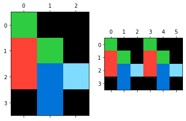
タイリング：16x128x128, 36x256x256, 25x512x512などが紹介されている。

色彩等の調整：augmentation：stain normalization：？

Maskデータの利用方法？

２．trainとinference

notebookをtrainとinferenceに分けるには、どうすればよいのか？inferenceだけで動作しているのは、訓練済みのパラメータをKaggleのデータセットとして保存しているのだろうか。

test.csvには、image_idのデータが3つしか入ってないが、どうなっているのだろう？

３．Karolinskaの論文に学ぶ

なんかスケールが違う。レベルが非常に高い！

1枚のスライドから1000パッチ：1パッチは598x598 ピクセル：30のInception V3からなるアンサンブルを2組用意：1組は悪性と良性の分類：1組はGreasonスコアの予測：Tesla P100 GPUが136台：組織の画像に組織のマスクとペンマークのマスクを重ねてラベルマスクを作成：

training：バッチレベルでラベルを付けて学習させる：スライドレベルでラベルを付けて学習させる：パッチ集合体にマスク情報を重ねて学習させる？：クラスアンバランスへの対応： 

7月3日：あと20日

１．Radboudの論文に学ぶ

こちらは、さらに高度というか、自動化を実用化するためのステップを確実に歩んでいる気がする。全てにおいて、非常に緻密にやっておられるし、1つ1つのステップが合理的でかつ正確に記述されているように思う。

自動化のためには、標準化が必須であり、標準化のためには信頼できる試料とラベル（正確な評価値）が必須である。ここに最も力を注いでいるのがRadboundであり、この論文で表現していることだと思う。

小さなメモ：deep learningとreference standardの不一致は、2と3の境界および4と5の境界を決めるところで生じているようである。confusion matricsでみれば明白。

augmentation: flipping, rotating, scaling, color alterations (hue, saturation, brightness, and constrast), alterations in the H&E color space, additive noise, and Gaussian blurring.

２．公開コードを動かしてみた。タイルを作成して、pretrainモデルで学習するものだが、1エポックに1時間以上かかっている。とりあえず、明日の朝まで動かしてみよう。途中で停止しないことを祈る。

7月4日：あと19日

朝起きると、プログラムが強制終了されていた。7エポック目の計算中に停止。連続使用可能時間は9時間となっているようだ。

今回走らせたコードの1回の訓練には、最低でも10エポック程度は必要で、15時間程度かかる。9時間で強制終了だと、1度の訓練回数を減らして、訓練を継続できるようにする必要がある。

たとえば、そういうプログラム変更は、使い慣れていないと難しく、書き換えるかどうか悩むところだ。

いずれにしても、Kaggle kernelだけでは不足なのと、自分の計算環境も使えることは必須なので、

ステップ１：自分の計算環境で同等の結果を得られるようにする。これができれば、まずは、fastai, pytorch, tensorflow/keras, のどれでも良い。

１．"git"がインストールできていなかった。conda install -c anaconda git

２．KaggleのデータベースにEfficientNet-PyTorchがアップロードされているのを知らなかった。Kaggle kernelからimagenetで学習したEfficientNet-PyTorchをつかうことができる。他に何があるか調べておこう。

３．Value Error! cannot decompress jpegが表示された。だいぶ時間をかけたが解決せず、scikit-imageのバージョンアップで解決するとの書き込みに対しては、condaがまだ対応していない。画像表示だけなので横に置いておく。

４．Kaggleのデータセットの使い方、パブリックデータセットスペースの使い方を学んでおこう。

・データセットとして、imagenetで学習済みのDNNのweightがアップロードされており、さらに、コンペのデータセットで学習したDNNのweightをアップロードしておいてKaggle kernelから呼び出してこれらのweightを読み込むことができるのだろう。この点に関して初心者につき確信無し！

・PANDA Challenge関係では、tileに変換した画像が何種類かアップロードされている。

・汎用的に使える、種々の学習済みCNNがPyTorch, Keras, fastai用にアップロードされている。そこに便利に使えるデータがある、というだけでなく、関連論文が紹介されていることもあり、丁寧な解説がついていたりすることもある。

５．データセットについて調べていてあらためて感じたのは、notebookの公開についてである。コンペなのに比較的性能の高いコードがコンペ中に公開されていて、借り物競争することに躊躇していたが、Kaggleのコンペが求めているのは、借り物でトップ50％レベルに入ることではないのだろう。たとえば初期のトップ20～50％くらいのコードを利用させていただいてsubmitすることでLBに顔を出し、そこからスコアを上げ、順位を上げていくことに注力する中で、先輩のコードに学び、試行錯誤し、成長していくことが期待されているのだろうということである。コンペにはいくつも参加してきたが、公開コードでLBに顔を出したのは、このコンペで3度目である。1度目は、後ろめたさを感じながら、借り物でLBに顔を出したものの、コードの理解が追い付かず、スコアアップの手がかりは得たと思ったが、コードに反映する技術が足りず、改善には至らなかった。最後の方はあきらめていたような気がする。2度目はTReNDSである。このときは、借り物からスタートして上位に進出したいと思って、積極的に公開コードを利用させていただいたが、結局は、そのスコアを超えられなかった。しかし、借り物をすると、そのスコアを超えたいという思いが強くなり、必死でコードを理解しようとするし、よりスコアが高くなる方法を探そうとするので、成長にプラスになると感じる。ということで、このコンペは、躊躇なく、公開コンペを利用させていただいてLBに顔を出した。さてさて、この先、どうなることやら。

６．重たい計算だから、TPUを使ってみよう！と思ったのだが、そんな簡単なものか。そもそも、TPUとGPUの違いはどこにあるのか。今回のコンペにTPUはうまくはまるのだろうか。batch_sizeを増やすにはメモリー不足かもね。

７．TPUの使い方、明日、勉強しよう。

7月5日：あと18日

１．TPUを用いたnotebook：42x256x256x3：.tfrecフォーマットのタイルデータを読み込み：GPUを用いたnotebook：36x256x256x3：学習中にタイルデータを作成

GPUを用いたnotebookは、タイルデータを作成しながら学習させているので、TPUとGPUの比較にはならない。

この2つのnotebookの最も大きな違いは、TPUを用いたnotebookは、トータルの処理時間が短いので、Kaggle kernel内で追試しやすいことかな。

２．TPUを用いたnotebookに学ぶ：トラブルシューティングを日本語に訳して眺める：動的形状がサポートされない：トレーニング速度とメモリー使用量を大幅に改善するため、グラフ内のすべてのテンソルの形状は静的、すなわちグラフをコンパイルする時点でその値が既知である必要がある：これを原因とするエラーが起きないよう、端数を削除するなどの命令が用意されている：計算効率を最大にし、パディングを最小限に抑えるようにメモリ内にテンソルをレイアウトしようとする：メモリのオーバーヘッドを最小限に抑え、計算効率を最大化するために、バッチサイズの合計は6の倍数、特徴ディメンションは128の倍数、などが良いらしい。：速度を上げるには、なにがしかの自由度を犠牲にする必要があるということのようだ。

３．Kaggle kernelのTPU環境でtrainingできそうなので、TPU/TensorFlow/KerasとTPUに合致したデータベースの組み合わせを使わせていただいて、モデルの予測性能を向上させる技術を検討することに注力しようと思う。

４．明日は。TPUモデルのtraining方法を検討してみよう。 

7月6日：あと17日

１．TPUモデルの検討は、エラー発生により中断。

TPUのメリットは、計算時間が早いことで、それは、Kaggle kernelを使用して大きなモデルのトレーニングをする場合には適合する場合もあるが、トラブルシューティングを読み込んでいくと、高い速度で計算するには制約条件が多く、その条件から外れると、期待した速度が得られないだけでなく、精度が低下することもあると書かれている。DNNは、もともと、計算時間が長いだけでなく、出力も安定しない。それを克服するための種々の工夫がなされているが、それがTPUと整合する保証はない。ゆえに、TPUは、それ自体を調査対象とすることには興味があるが、コンペでは、その計算速度の高さが、モデルの予測性能の向上につながらなければ意味がない。

いま発生しているエラーは、上記の事情とは無関係だが、諸条件を勘案し、TPUモデルの検討は、中止する。

２．次の実験計画：

Kaggleデータセットにあるタイル画像と、imagenetで学習済みのefficientnetを用いて、transfer learningのモデルを作成し、自前の環境で、計算時間、計算精度を調べる。

TensorFlow/Kerasを使う。

３．公開notebookに学ばないとだめだ。

・目標とするnotebookを１つに定めて、最後まであきらめずにスコアアップに努める中で、コードを学ぶ。

・新しい活性化関数といえば、'elu'かと思っていたら、'Mish'が良いらしい。

・augmentationを個々のタイルと結合したタイルの両方でやるのか？

・transfer learningとfine tuning、考え方、やり方は難しくないが、データにうまく適合させるには、やはり、何かが・・・。

only one DO(0.5) and small augmentation parameter

only one DO(0.5) and small augmentation parameter

ひどいオーバーフィッティングだ！

・PyTorchの転移学習は、モデル（たとえば、最後の全結合層など）が見当たらないのだが、どうなっているのだろう。（PyTorch素人発言です）

DO and BN

DO and BN

 今度は、regularizationのやりすぎか。

7月7日：あと16日

１．上記のregularrizationやりすぎのような結果になった理由がわかったような気がする。A. Geronさんのテキスト341ページに次の記述がある。Finally, like a gift that keeps on giving, Batch Normalization acts like a regularizer, reducing the need for other regularization techniques (such as dropout, described later in this chapter).

つまり、Batch NormalizationとDropout(0.5)のセットを最終段で、2回使っていたのだ。さらに、augmentationの変化幅を大きくしていたのである。

２．これを確認しよう。

実験１：2か所のDropout(0.5)を取り除く。

実験２：2か所のBatch Normalization( )を取り除く。2か所のDropout(0.5)は復活。

これで、Dropout(0.5)の寄与とBatch Normarizationの寄与がわかるだろう。

DO use BN not use

DO use BN not-use

BN use DO not use

BN use DO not use

＊GPU使用可能時間が少なく、エポック回数を5回に減らしたので、DOとBNの両方を同時に使ったときとの比較は、少しやりにくい。

・BNよりもDO(0.5)の方が、汎化能力は高いようだ。

・BNの汎化能力は、高くはなさそうだ。

＊前途多難：小さな改善検討では、とても上位には行けない。しかしながら、この小さな改善を正しくやるのは、とても難しいのだ。

＊根本的な改善方法の探索が必要だ。どうやって探す？

7月8日：あと15日：

Kaggle kernelのGPU残り時間25分（スイッチ切り忘れにより15時間のロス、11日の午前9時まであと3日間は使えない）

１．実験３：昨日の続きで、Dropout(0.5)とBatchNormalizationの両方とも外してみた。

no DO and no BN

no DO and no BN

・今回の実験の結果をながめての結論は、明確ではないが、BNとDOの両方を使って、かつ、DOの割合を追加調整する、ということになるかな。それから、できれば10エポックぐらいまで計算したかったが、GPUをoffにするのを忘れて、できなくなった。

２．転移学習再考：

かっこつけて、再考と書いてみた。その意味は、テキストで学習しているだけでは身に付かない、実地で経験しながら検討しよう、ということです。しかし、GPUが使えないので、土曜日までは、実験できない。

A. Geronさんのテキストの10章に、ヘアスタイルを識別する場合、顔認識のためにトレーニングしたモデルがあれば、ランダムパラメータからスタートするより、顔認識の学習済みモデルの入力側に近い層のパラメータを初期値にする方が早く良い結果が得られる、というようなことが書かれている。

11章には、Fashion MNISTを題材にして、転移学習の1つの手順が示されている。ここでのポイントは、学習済みモデルの出力層のみを取り換えること、最初の数エポックは、再利用するパラメータが壊されないように固定しておくこと（layer.trainable = False）、その後でtrainableにするのだが、再利用するパラメータが破壊されてしまわないように、学習率をデフォルト値よりもかなり小さくすること（説明事例では1/100）、などであろう。

最後に、14章には、imagenetでpretrainしたXceptionを用いた花の分類例。花の画像が1000枚、すなわちデータ数が少ない場合の活用例。最初に、練習用のデータセットをtest_set, valid_set, train_setに分けている。次にモデル（Xception)の入力データサイズ224x224に合わせる。tf.image.resize(image, [224, 224])。さらに、shuffle, batching, prefetching, augmentationなどのpreprocessingをする。肝心のモデルだが、imagenetで学習したモデルとパラメータをロードする。必須条件は、include_top = False。これは、global average pooling layerとdense output layer（imagenetは1000種類に分類するから、1000のユニットからなる）を除去することで、代わりに、自前のglobal average pooling layerと、分類数のユニットをもつdense output layerを追加する。trainingの最初はbase_modelをlayer.trainable = Falseとして、数エポック、続けて、base_modelをlayer.trainable = Trueとし、かつ、learning rateを小さくして学習させる。およそこんな感じだ。

３．F. CholletさんのテキストにおけるTransfer learning

関連する内容は、Using a pretrained convnetで始まり、feature extractionとfine-tuningという表現になっていて、transfer learningという用語は、少なくとも見出しには使われていない。全体がTransfer learningで、バリエーションが多いという感じがする。

４．NIPS 2019の論文

Transfusion: Understanding Transfer Learning for Medical Imaging
Maithra Raghu∗ Cornell University and Google Brain maithrar@gmail.com
Chiyuan Zhang∗ Google Brain chiyuan@google.com
Jon Kleinberg† Cornell University kleinber@cs.cornell.edu
Samy Bengio† Google Brain bengio@google.com
Abstract
Transfer learning from natural image datasets, particularly IMAGENET, using standard large models and corresponding pretrained weights has become a de-facto
method for deep learning applications to medical imaging. However, there are fundamental differences in data sizes, features and task specifications between natural
image classification and the target medical tasks, and there is little understanding of
the effects of transfer. In this paper, we explore properties of transfer learning for
medical imaging. A performance evaluation on two large scale medical imaging
tasks shows that surprisingly, transfer offers little benefit to performance, and
simple, lightweight models can perform comparably to IMAGENET architectures.
Investigating the learned representations and features, we find that some of the
differences from transfer learning are due to the over-parametrization of standard
models rather than sophisticated feature reuse. We isolate where useful feature
reuse occurs, and outline the implications for more efficient model exploration. We
also explore feature independent benefits of transfer arising from weight scalings. 

医療データの解析にtransfer learningがデファクトスタンダードとして用いられていることに意義を唱えている。疑問点は、たいていの人が感じているように、imagenetと医療画像とでは、画質も読み取る情報の位置や分布なども全く異なるので、そもそも、imagenetで学習したモデルのtransfer learningに大きな効果を期待するのはおかしいのではないか。transfer learningの効果があるとしたら、その理由、根拠は何なのかを、実験的、具体的に示したデータがあるのか。著者らは、確かに高い性能を示しているが、それは、transfer learningから期待されるもの、特徴量の効果的な利用、などによるものではなく、単にモデル自体の性能の高さによるものであろう、というのがこの論文の結論のようである。その根拠を示す結果を得ているようだが、自分にはそこまで読み取れない。

仮に、この論文の結論通りだとしても、imagenetで学習した高性能なモデルを用いることは、他の初期値を用いるよりも収束が早くて期待通りの性能が得られることに間違いはないのだから、我々は、何も変えることはない、ということになるのかな。

５．モデルのもつ性能を生かすための方法を考えよう。

病巣の面積率を反映した評価になるようにするには、タイルの集合体の中に組織の全体が入っているほうがよさそうだし、ある程度の画質も必要だし、モデルの性能は高い方がよさそうだし、計算時間の制約もあるし、・・・。

明日も、Kaggle kernelのGPUは使えないので、頭を使わないとだめだな。 

7月9日：あと14日：

１．タイルの作り方を学ぶ：タイルの枚数、組み合わせ、各タイルの視野と解像度、これらを自由に操れるようになるため。

解読中

２．出力層をシンプルにしてみた。

・GPUが使えないので、CPUで動作確認したところ、オーバーフィッティング気味に動作することがわかった。

・そうすると、augmentationをしっかりしないといけないので、albumentationを調べてみた。非常に種類が多いことが分かった。これまで使ったことのないものについて、１つ１つ効果を調べてみる。

 明日は、タイル作成コードをしっかり理解して、思い通りのタイルが作れるようにしよう。

7月10日：あと13日：

１．タイル作成コード：

・画像の高さと幅の値を取得する：例：image_shape = image.shape

・タイルの画像サイズをtile_sizeとしよう。

・元画像にパディング（周囲にダミー画素を追加）する。パディングは、パディングした画像サイズが、tile_sizeの整数倍になるように行う。

・パディングの大きさ（各方向へのピクセル数）を計算するために、演算子%が使われ、パディングを上端下端、左端右端に振り分けるために//2が使われる。

%や//の入った演算は、わかってしまえばどうってことないが、初見では戸惑うこともある。そういうときは、元画像の画素数とタイルの画素数を式に代入して、作図してみよう。数式は、具体的数値を代入し、その結果を図やグラフに表すと理解しやすい。

・.pad, .reshape, .transpose, .argsort, 等を、通常の説明書レベルで理解するだけではだめなのだろうという気がする。実際、np.padなども、説明書とは異なるフォーマットでも使われているようで、どう理解したらよいのかわからない。

・以上の結果、自分で組み立てなおしたり、欲しい解像度、形状、のタイルを得るのはあきらめた。使わせていただいているプログラムは、制約はあるものの、自由度は高く、さまざまなタイル構造を作り出すことができる。

明日は、何種類かのタイルの比較を行う予定。

7月11日：あと12日：

自分でコントロールできるプログラムは、いまだ、LB: 7.0にとどまっている。

discussionでの上位者の含蓄のある発言：要約すると、「実験あるのみ！」

タイルの解像度と枚数の制御範囲は広がった。そうすると、ある程度の解像度で検体全体を含むタイルを使いたくなるのだが、計算資源の問題にぶつかってしまう。

解像度の高い画像が得られたので期待して動かしてみた。ただし、バッチサイズ２でしか動かない。計算時間が長い。モデルとフィットすれば数エポックで高いスコアも可能だと期待して途中経過を見ていたが、予想外に悪かった。タイル画像は明瞭で、これなら容易に分類できるだろうと思っただけに残念だった。

自分の目を、コンピュータに合わせないとだめだな。実験あるのみ。先入観なしに、系統的に、実験しないといけないようだ。

検討中のモデルを、今朝、GPUを用いて10エポック計算し、スコアは0.75くらいだったのでcommitしたが、9時間も経ってエラーで停止し、スコアは得られなかった。lossやaccのデータまで消えてしまった。非常に残念だ。

もう1つのモデルも計算しているが、commitできるか心配だ。

心配どおり、今度は、自分でミスった。

はい、今日は、終り。

7月12日：あと11日：

勝者のキーワード：

Kaggle kernel、private dataset、GPU、TPU、の使いこなし。

stacking、ensemble、concatenate、・・・。

このあたりを調べてみよう。

・タイルの構成（個別タイルの解像度と画像範囲）を整えると、やたら画像が大きくなることがある。そのときは、適度な大きさにリサイズする。これを正しく行うためには、データの流れを正しく把握しなければならない。そのためには、プログラムを正しく理解しなければならない。もう少しだと思っている。

・どのタイルが良いのかを試しながら、良さそうなものを組み合わせる。アンサンブルの登場だが、出力をどうするのか。まだ理解していないので、見本になるプログラムを探して、学ばなければならない。

・各クラスに特徴的な画像を機械学習で抽出し、それを用いてCNNで学習させるというのが面白そうだし、CNNを通して特徴量を抽出してから機械学習で分類するのも面白いかもしれない。ただし、これは、単なる思い付きにすぎず、素人の妄想にすぎないかもしれない。。

・Kフォールドをやって、学習済みの各モデルで予測したクラスの平均をとるか、予測したクラスの多数決をとるか、これも妄想かもしれない。

・今日もcommitのところで、時間切れで失敗した。コミットがうまくいったのは借り物の予測・提出用のプログラムと、これも借り物だが、約3時間かかって計算した後、GPUをonのままにして約3時間でcommitしたものだけだ。

後者のkommitのとき、GPUは、3時間くらいしか動いていなかったはずなのに、その3時間の間にGPUを15時間くらい使ったことになっていたような気がする。

まだ20時間あると思っていたのに、残り5時間の警告が出てあわてて動作中のプログラムがないか調べて対処したように思う。

いまだに、コミットのときの条件を正しく把握できていないのだろうと思う。うまくいかなかったのは、2回とも、計算終了後にGPUをoffにしたことが原因だろうと思う。

commitの際に、GPU使用時間のさらに3倍以上の使用時間を消費してしまった原因は、コミットに要する時間が長くて、コミット中に、別のプログラムを編集しようとしてkernelを立ち上げた際に、GPUがプログラムに同期して自動的に立ち上がっていたのに気づかなかったためだろうと思う。

まだまだこんなレベルなのだ。

計算用と予測用を別にするなど、kernelを効率よく使う方法を習得したいものだ。

commitしたところで、良くてもLBは0.75くらいだろうからGPUを無駄に使わずに済ませられないかと思ったのも事実だ。

忘備録：技術習得目標

➂アンサンブル：異なるCNN、異なるフォールド、異なるタイル構造、異なるハイパーパラメータ：計算環境の問題

④学習の継続：引継ぎ：学習モデル（学習パラメータ）の受け渡し：学習と予測の分離：学習モデル（学習パラメータ）の受け渡し：それほど必要性を感じていない：それではだめだ。これは、自在にできるようにしておかなければならない。

②タイル等の画像のリサイズ：入力画像の画素数の調整：配列の次元が多い場合に対応できない：次元の低い話だ。 

①自分の計算環境でどのnotebookも動かせるようになること：これがいつまでたっても克服できない ：windowsからlinuxに切り替えることで解決できるのだが、いつまでも、踏み切れずにいる。

7月13日：あと10日：

アンサンブルに限らないが、使いたいデータは、KaggleのDatasetsのpublicもしくはyour detasetsにアップロードしておき、Kaggle kernelのnotebookから、それらをアップロードするという使い方がある。

複数のモデルに対する学習済みDNNの重みをアップロードしておくことで、アンサンブルが容易になる。

強力なマシンを使って学習させたモデルの重みをアップロードすれば、それだけ予測精度の高いモデルを使うことができる。

容量制限はあるが、データベースもアップロードできるので、時間をかけて前処理したデータをアップロードしておくこともできる。

出力層：すでに書いたかもしれないが、現時点では、GlobalAveragePoolingの後は出力層に直結している。これで良いのかどうか、わからない。出力層としてdense層を加えた場合と比較しだすときりがないと思うので今はやらない。

学習済み（もしくは学習中）モデルのsaveとload、callbacks、modelcheckpointやearlystoppingなどは、ディープラーニングのテキストを読んで勉強しているときは、読み飛ばしていたように思う。

trainingに時間がかかるDNNでは、このあたりを押さえておかないと、時間を無駄にしてしまっていることを、実感させられているところである。

ここのところ、ずっと、毎回、imagenetで学習したモデルからスタートしてtrainingしているが、何か無駄をしているような気がしてならない。

モデルは学習するたびに賢くなっていくべきだと思う。さまざまに学習した成果を蓄積する方法はないものだろうか。

面白い論文があった。

Automated Gleason Grading and Gleason Pattern Region Segmentation Based on Deep Learning for Pathological Images of Prostate Cancer. YUCHUN LI et al., IEEE Acsess 2020

明日読んでみよう！

このコンペの技術目標を、「アンサンブルモデルによる予測」ということにする。

まだ、あと、9日間もある。

7月14日：あと9日：

学習と予測の分離及びアンサンブルを行うための枠組み：

（学習コードアップロード⇒学習⇒モデル保存）＊ｎ⇒予測コードアップロード⇒ｎ個のモデル読込（＋アンサンブル）⇒予測

ここで、保存したモデルは、Datasetとして保存する。予測コードをアップロードしたら、Datasetとして保存したモデルをアップロードする。

学習と予測の分離、および、DNNのアンサンブルの枠組みを理解するのに、14日間を要した（Kaggleに参加したのは昨年の今頃だったと思うので、1年を要した）。理解が正しいかどうか、簡単なモデルを使って、確かめてみよう！

Dropout：次の論文は、非常に重要で、参考になることが書かれているのに気づいた。主題は「isometric」であるが、自分にとって最も参考になりそうなのは、著者らが提案しているモデルに「dropout」を追加するだけでResNetの性能に近づいた、というところである。

今使っているモデルがoverfittしたら、同じ場所に、追加してみよう。

dropout(0.4)で効果はあったが、まだ不足。入力データの量とモデルの複雑さのバランスがとれていないのだろうが、適正化は時間がかかる。限られた時間と計算資源を有効に使って・・・。

Deep Isometric Learning for Visual Recognition
Haozhi Qi, Chong You, Xiaolong Wang, Yi Ma, and Jitendra Malik          arXiv:2006.16992v1 [cs.CV] 30 Jun 2020
Abstract
Initialization, normalization, and skip connections are believed to be three indispensable techniques for training very deep convolutional neural networks and obtaining state-of-the-art performance. This paper shows that deep vanilla ConvNets without normalization nor skip connections can also be trained to achieve surprisingly good performance on standard image recognition benchmarks. This is achieved by enforcing the convolution kernels to be near isometric during initialization and training, as well as by using a variant of ReLU that is shifted towards being isometric. Further experiments show that if combined with skip connections, such near isometric networks can achieve performances on par with (for ImageNet) and better than (for COCO) the standard ResNet, even without normalization at all. Our code is available at https://github.com/HaozhiQi/ISONet.

Table 5

Since R-ISONet is prone to overfitting due to the lack of BatchNorm, we add dropout layer right before the final classifier and report the results in Table 5 (g). The results
show that R-ISONet is comparable to ResNet with dropout (Table 5 (b)) and is better than Fixup with Mixup regularization (Zhang et al., 2018).

CNNのアンサンブルができるようになっても、今のモデルでは、単独で、まだ0.75を超えていないので、アンサンブルがうまく機能しても、LBは0.8にも届かないだろうな。

単一モデルで少なくとも0.85以上にならないと、勝負にならないだろうな。

分類のところに注目してみようか。

病巣の段階とその検体中における占有面積比が重要な意味をもっているように思う。

そうすると、タイル画像内で、病巣の占有率が把握できるようになっている必要がありそうだ。すなわち、タイルには、各検体の全体が写っていなければならないのではないか。クロップなどのaugmentationによって画像が画面からはみ出して見えなくなるのはまずいだろうな。元々のタイル内に、検体全体が含まれているのが大前提となるのか。

さて、今週のGPU使用可能時間は、あと4時間半となった。今走らせている計算が終われば残りは1時間となる。あと3日半は、GPUが使えない。

ということで、残っている大きな課題の１つである、自分の計算環境の整備をこの3日半の間に片付けてしまおう。

Anacondaの仮想環境を、元の環境をコピーして作成し、そこに、pipで必要なモジュール等をインストールすることで、たいていのものは動くようになる。さらに、Kaggleの議論もさんこうにしながら進めている。

これでOKかと思ったら、こういうエラーが出た。”BrokenPipeError: [Errno 32] Broken pipe”　この原因が、さっぱり、わからない。これはPyTorchのモデルだ。

この作業をすることによって、Kaggleのpublicデータセットの使い方が少しわかった。

明日は、なんとしても、BrokenPipeErrorを克服しよう！ 

7月15日：あと8日： 

BrokenPipeError：

定義：exception BrokenPipeError 

A subclass of ConnectionError, raised when trying to write on a pipe while the other end has been closed, or trying to write on a socket which has been shutdown for writing. Corresponds to errno EPIPE and ESHUTDOWN.

日本語バージョン： 

ConnectionError のサブクラスで、もう一方の端が閉じられたパイプに書き込こもうとするか、書き込みのためにシャットダウンされたソケットに書き込こもうとした場合に発生します。 errno EPIPE と ESHUTDOWN に対応します。

・なんのことやらさっぱりわからん。

・そこで、エラーメッセージの中を１つづ追いかけてみる。どうやら、data.to(device)のところがあやしい。deviceは、GPUである。

・パソコンに搭載されているGPUは1050Tiなので、メモリーは４GBである。そうすると、pytorchでは、num_workers = 0　以外の選択肢はなさそうである（pytorch GPU num_workersをキーワードに検索してみると、それらしい説明があった）。tensorflow/kerasでは、num_workers = 4でエラーが発生したときに、たぶん、num_workers = 1で動いたと思う。今回も、最初にnum_workers = 4があやしいと思って4を1に変更したが、エラーは発生したままだった。

・なにはともあれ、エラーの原因は、num_workersの値が、使っているGPUとマッチしていなかったということである。適正な値を用いることで、エラーは解決した。

・エラーの原因は、元プログラムが想定しているよりもGPUの能力が低いことにある。したがって、トップを狙える可能性は、いまだ低いままである。

・今、ノートパソコンのGPU:1050Ti:の冷却ファンがうなりを上げている。

・2エポックでval_kが0.68くらいまで上がりそうだったので、よしよし、と思っていたら、2エポックで停止、3エポック開始時にエラーが発生した。

・まいった、まいった。

・2エポックの計算に3時間以上かかっているので、エラー対策をしてもその結果がわかるまでに、３時間以上かかることになる。

・類似エラーのQ&Aには、pytorchのバージョンを最新のものにすればよいとか、1つ前のバージョンにすればよいとかいうのがある。現状は1.2だから、まずは、1.4にして、それでだめなら、1.5にしてみよう。これで結果がわかるまでに7時間以上かかることになる。2エポックまでは計算できるので、タイルの条件を変えてみよう。

コンペサイトの説明で気になる箇所がある。

１．training setのイメージの一部は、ペンによりマーキングされているが、test setにはマーキングはない。

２．セグメンテーションマスクが用意されていて、ISUPグレードが示されている。全ての画像に付属しているわけではない。種々の理由により偽陽性、偽陰性が含まれている。マスクは、効果的なサブサンプリングをする方法を開発するのを支援するために提供したものである。マスクの値は供給機関によって異なる。

３．機関によってラベル（の定義）が異なっているようにみえる。

技術検討用ということでしょうか。最初はマスクを使わず、写真や試料の不具合も関係なくそのままデータを通す。次からは、不具合のある写真や試料を除く。試料がどちらの機関由来かを識別することができるかどうか調べる。テストデータについても機関間の識別ができれば、機関ごとに学習モデルを作りテストデータを分類することができるかもしれない。どれがうまくいくかは、予測結果を提出してスコアが算出されるまでわからない。 

計算環境の問題：

仮想環境(????vision)を作ったうえで、condaでインストールできないモジュールやパッケージをpipでインストールしている。

仮想環境のpytorchを1.2から1.4もしくは1.5にバージョンアップするつもりが、まちがってベース環境のpytorchをバージョンアップした。

notebookをどちらの環境で立ち上げているのか間違うと、環境を壊してしまうことになりかねないので要注意。

出来ることが増えるということは、管理すべきことも増えるということ。

使い方がわかっていないところがある。

pytorchのバージョンアップが、jupyter notebookに反映されない。 

明日は、このエラー対策だ！

AttributeError: 'CosineAnnealingLR' object has no attribute 'get_last_lr'

これも！

pytorchのバージョンアップが、jupyter notebookに反映されない。

エラーに明けて、エラーに暮れる。

そうだ！　AIエンジニア＆AI研究者になろう！

7月16日：あと7日：

今日の課題は、1.2.0から1.4.0以上へのpytorchのバージョンアップ：

Anacondaを使用している。

conda updateから始めたのだが、1.2より新しいものが出てこない。uninstallしてからinstallしても、1.2.0だけを推奨し、バージョンアップできない。アップデートや再インストールの際にバージョンを指定しても、別の場所に、単独でインストールされるようで、使える状態にはならない。conda listでは1.2が表示されるだけである。

condaによるfastaiのインストールの説明文の中に、pytorchへの言及があった。Anacondaにはfastaiもインストールしているので、非常に気にはなったが、pytorchのインストールやバージョンアップへの影響に関係する記述はないようだ。

試しに、fastaiとpytorch 1.2の両方をアンインストールしてから、pytorchのみインストールしようとしたが、1.2しか出てこない。

pytorchのHPに書かれているインストール方法、conda install pytorch torchvision condatoolkit=10.2 -c pytorchを実行してみた。もう３時間近く動いている。互換性のないパッケージを調査するということで、examining conflict for ... が表示され、動き続けている。もう5時間以上になる。これだけ時間がかかると、うまくいくとは思えない。pytorchはtensorflow/kerasと衝突しているのだろうか。もう10時間を超えただろうか、延々とexamining conflict forが続いている。これでバージョンアップできたらAnacondaの技術者は凄いってことになるのだが。どうかな。

1日つぶした。pytorchのバージョンアップが目的なのではなく、エラーが生じた可能性の１つがこれではないかということである。エラーが生じているのは、learning rateの更新のところだから、プログラムの変更でエラーはなくせるかもしれないので、そちらをやろう。

7月17日：あと6日： 

Kaggle kernelに頼りすぎたな。もっと広く言えば、Kaggleのコミュニティーに頼りすぎたな。技術を磨くには、とても良い仕組みであり、コミュニティーだと思う。引き続き利用させていただきたいと思っている。自分にとってのメリットとデメリットを列挙してみよう。

メリット

・スコアを争うことは、真剣に取り組む動機付けになる。

・スコアを争うことにより、モデルの予測能力を上げるための技術に敏感になる。

・スコアを争うことにより、当該分野の技術開発状況に敏感になる。

・公開コードによって、プログラミング技術の基礎から、モデルの高性能化のための様々な工夫、様々なデータの前処理技術を学ぶことができる。

・自前の計算環境が無くても、Kaggle kernelで、GPUやTPUを使うことができる。

デメリット

・公開コードに頼りすぎると、自前のコードを作らなくなってしまう。

・Kaggle kernelに頼りすぎると、自前の計算環境の保守がおろそかになる。

 さて、あと6日になった。

ハイスコアを狙うには、1050Tiは自分の能力との足し算では、不足である。

自分が或る程度理解できて、ある程度条件検討してきた中で、最も良いスコアが得られそうだと思うタイルとモデルの組み合わせにおいて、良いスコアを出すために必要な時間は短く見積もっても100時間である。残りは30時間である。4週間前なら120時間あるが、今使っているモデルは自前ではできないノウハウが入っており、その時期にそのモデルの原型が公開されていても自分ではとりかかれていないだろうと思う。

google colaboは使えるのかどうか調べてみよう。

Kaggle kernelよりも一般向けに設計されているようである。使えるGPUやTPUの性能は同レベルかな。Google Driveは15GBまで無料で使用可能。12時間まで連続使用可能となっているようだが保証されているわけではない。

大容量のデータや大きなモデルを扱うためには、Google Cloud Platformを使うことになるのだろうな。自前のモデルで、ハイスコアの可能性があれば、やってみてもよいのだが、・・・。

最後までスコアアップの手段を検討し続けよう！

7月18日：あと5日：  

ハイスコアのポイント：

データの特徴：2つの機関KとRから、データとラベルが提供されている：ラベルにも画像にもバイアスがかかっている：Kの画像/ラベルで訓練したモデルでKのテスト画像のラベルを予測し、Rの画像/ラベルで訓練したモデルでRのテスト画像のラベルを予測するのが最も正確だと考えるのが妥当だろう：入れ違いになるとどうなるのだろう：Kの画像/ラベルで訓練したモデルでRのテスト画像のラベルを予測し、Rの画像/ラベルで訓練したモデルでKのテスト画像のラベルを予測した場合が最も不正確になると考えるのが妥当だろう：KとRの論文には、正確なラベルを与える難しさが書かれている：不正確なラベルが、ある割合で含まれている：コンペの概要には、ラベルの定義すら違っているような記述がある：Rでは試料をいくつかのクラスに分けてラベル付けしている：そのクラス/ラベル付け手法によってラベルの正確さは異なっている：そのうちのどれが訓練データに、どれがテストデータに組み入れられているのかは不明：機械学習を援用して半自動でラベル付けしたり、専門家がラベル付けを繰り返したり（不一致のラベルは再検討）している。加えて、不良データの追加、マスク（セグメンテーション？）の付与、マーキング残しなどがある：こういう状況の中から、テスト画像に付与されたラベルを予測する：主催者の期待はどこにあるのだろうか：少なくとも、テストデータのラベルは、専門家による最も確度の高いものでなければ意味がないと思うが、現実にはグレーゾーンがある。ミスもある。意図的にノイズデータを加えることもある。：もし、最初に述べたとおりになっているのなら、訓練データを用いて、徹底的にRとKを識別するのがよくて、そのモデルでテストデータをRとKに仕分けし、対応する訓練モデルで予測するのが最も正確な予測結果をもたらすのかな：そうだとしても、用いるDNNモデルが貧弱であったり、タイリングなどの画像の前処理技術が貧弱であったり、計算資源が不足していれば、高いスコアは望めない。

機械学習プログラムの設計製作技術を身に着けよう、向上させよう、絵に描いた餅に終わらないようにしよう！

さて、Kaggle kernelのGPUの最後の30時間を有効に利用する方法を考えよう。

今回のコンペで新たに学んだのは、Kaggle Datasetの利用/活用方法である。これを使って３つか4つのCNNモデルのアンサンブルを試してみることにする。

7月19日：あと4日：   

アンサンブルを1回やって今回のコンペは終えることになりそうなので。効果的なアンサンブル法についてコンペ内での情報があれば参考にしながら考えてみたい。

アンサンブル用予測モデルの取り出しに失敗した。

明日は、目標を小さくするしかない。

予測モデルの取り出しだ。

自分の今のレベルがよくわかった。

7月20日：あと3日：   

今日は全休です。

7月21日：明日提出締切（正確にはあさって午前9時00分まで） 

 今日の予定：次のステップへの準備

１．Kaggle kerner内での出力ファイルの確認と取り出し

２．Kaggle kernelのGPUとTPUの活用について

結果

１．訓練中の出力ファイルの変化の確認、訓練終了直後の出力ファイルの確認、出力ファイルの取り出し作業を、1ステップ毎に記録しながら慎重に作業する

・計算途中であるが、これまでの最も良いモデルのパラメータファイルが出力されているのを確認し、ダウンロードできることも確認した。

・明日は、ダウンロードしたパラメータファイルをDatasetに保存し、予測用のコードに読み込んで実行し、submitしよう。

２．TPUを用いたnote bookから、TPU使用方法を学ぶ

基礎学習

Google Cloudからのコピペ

Cloud TPU は、Google がニューラル ネットワークのワークロードに特化して設計した行列プロセッサです。TPU では、文書処理、ロケット エンジンの制御、銀行取引といった操作に対応できませんが、ニューラル ネットワークの大規模な乗算と加算に関しては、極めて高速に処理でき、しかも、消費電力と内部の物理フットプリントは CPU や GPU と比較して大幅に下回ります。

TPU が他のデバイスより優れている点としては、フォンノイマン ボトルネックが大幅に軽減されることが挙げられます。このプロセッサの主要なタスクは行列処理であるため、TPU のハードウェア設計者はその演算処理の実行に必要なあらゆる計算ステップを把握しました。そしてその知識を基に、何千もの乗算器と加算器を配置して直接相互に接続し、これらの演算子からなる大規模な物理行列を形成することができました。この構造は、シストリック アレイ アーキテクチャと呼ばれています。Cloud TPU v2 の場合、128 x 128 のシストリック アレイが 2 つあり、16 ビットの浮動小数点値を処理する 32,768 個の ALU を単一プロセッサ内に集約しています。

・調べた範囲では、モバイル用途の他には、特段のメリットは無さそうだが、実際に使ってみなければわからない。2か月ほど前に、Flower Classification with TPUsというコンペがあったので、合間を見て、そこのnotebooksで学んでみよう。

明日は最終日だな。１つは、commitしてsubmitしよう！ 

7月22日：本日提出締切日（明朝午前9時）

本日の予定

１．最後のsubmit

・trainモデルを走らせ、最良のcvが得られたモデルのパラメータセットをsaveする⇒そのファイルをdata setとしてアップロードする⇒data setを経由して予測モデルにそのパラメータセットを読み込み、test dataの分類をしてsubmission fileを出力する。

・この手順でsubmitした結果、スコアはLB=0.85であったが、このスキームでsubmitする手法を学んだということで、良しとしよう。わずか4エポックの単一モデルでこのスコアが出るということは、元のプログラムがハイレベルだったということだろう。

２．commit中のGPU使用時間の確認

Kaggle kernel内での操作に少し慣れてきたので、以前から気になっていたcommit中のGPU消費時間を、commit開始からモニターしている。

現状の理解：

commitは、プログラムを再度走らせるので、GPUを使って5時間かかったのであれば、commitにもGPU使用で5時間かかる。（CPUでは計算に9時間以上を要する場合、GPUをoffにしてcommitすると、commitは失敗する）

GPUの使用時間は、GPUのon/off操作の下段にGPU Quotaとして表示されている。それを見れば、GPUの使用時間がリアルタイムでわかる。

commit中、GPU Quotaの時間表示は、session on/offによらず、実際の経過時間の倍の速さで時間は進む。

session onでcommitすると、GPU Quotaの表示のとおり、実際の経過時間の２倍の時間、GPUを使ったことになる。

session offでcommitしても、GPU Quotaの表示は2倍の速度で進むが、My account画面に表示されるGPU消費時間は、commitの経過時間のみを反映したものであり、 Quotaをクリックすると、やはり、commitの経過時間のみを反映した表示があらわれる。

画面によって異なる時間が表示される。これは、現実におきていることである。

しつこいようだが、GPUの残り時間から、commitできると思っていても、単純な操作ミスによって、commitに失敗することがあることに注意しよう。

注意）GPUのon/offと、sessionのon/offは、まめにチェックしよう！

３．data augmentationについて

train、validation、testの3つのステージについて考えてみる。

A. Geronさんのテキストでは、AlexNetの説明のところで、Augmentationが紹介されている。AlexNetはoverfittingを防ぐためのgenerarization techniqueとして、DropoutとともにAugmentationを用いていたことが紹介されている。

F. Cholletさんのテキストでは、データが無限にあればoverfitは起きない。その代替方法として、データをランダムに加工することによって本物に近いデータを増やす方法としてAugmentationを位置づけている。さらに、data augmentationは、所詮、元画像の単純な加工に過ぎずoverfitthingを防ぐには十分でない。その場合には分類器の全結合層の手前にdropout(0.5)を入れるとよい、と説明されている。

さらに、コードの説明のところで、validation dataに対しては、Note that the validation data shouldn't be augmentedと書かれている。

ということで、data augmentationは、train dataに対してのみ行うものと思っていた。

しかし、Test Time Augmentationは、適切に用いれば大きな効果を発揮する可能性があるようだ。次のような論文がある。

Greedy Policy Search:A Simple Baseline for Learnable Test-Time Augmentation

Dmitry Molchanov, Alexander Lyzhov, Yuliya Molchanova, Arsenii Ashukha, and Dmitry Vetrov, arXiv:2002.09103v2 [stat.ML] 20 Jun 2020

Test-time data augmentation—averaging the predictions of a machine learning model across multiple augmented samples of data—is a widely used technique that improves the predictive performance. While many advanced learnable data augmentation techniques have emerged in recent years, they are focused on the training phase. Such techniques are not necessarily optimal for test-time augmentation and can be outperformed by a policy consisting of simple crops and flips. The primary goal of this paper is to demonstrate that test time augmentation policies can be successfully learned too. We introduce greedy policy search (GPS), a simple but high-performing method
for learning a policy of test-time augmentation. We demonstrate that augmentation policies learned with GPS achieve superior predictive performance on image classification problems, provide better in-domain uncertainty estimation, and improve the robustness to domain shift.

・TTAは、予測性能を上げるための手法として過去に検討されていたようだ。

・Kaggleでは、すでに常套手段になっているようである。効果的なTTAを探そう。

４．今回、アンサンブルをやろうとしてできなかったこと

・アンサンブルのコードをどのように仕上げるかということも課題であったが、どういうアンサンブルをするのかを、決めることについても十分な検討はできなかった。したがって、効果のほどはわからないが、以下のような単純な方法を検討しようとしていた。

・タイルの枚数や解像度を変えたモデル

・学習率の初期値を変えたモデル

・パラメータの初期値（He、ランダム、imagenetによるpretrain）を変えたモデル

スコアアップのためのTTAを検討し、TTAを変えたモデルのアンサンブルというのもありかもしれない。

・GPUの残り時間が少ない中で、アンサンブルのためのデータ保存とそのダウンロードのタイミングを間違えたのが痛かった。

これで、PANDAコンペは終了だ！

目標の1位からは、はるか遠くの順位にとどまり、仮の（借り物の）スコアから抜け出せなかった。

次は、SIIM-ISIC Melanoma Classificationに取り組もう！

7月23日：本日午前9時終了

verify中とのことだが、最終結果が発表された。

＊順位について

まず、順位変動の大きさに驚いた。test_dataの42％を使ったPublic（暫定）から、残り58％のtest_dataを使ったPrivate（最終）とで、こんなに順位（スコア）が違ってもいいのか、ものすごく、大きな疑問を感じる。

200も300も飛び越してベストテンに入った人はおめでとうでよいのだが、優勝だと思っていた人が41位にまで下がっているのはなんとも残念な気がする。

＊上位の方々の戦術

印象に残ったのは2つある。

１つは、丁寧なラベルと画像の選択である。これは、ディープラーニングの基本中の基本、すなわち、良い（画像 - ラベル）ペアを作り上げることである。この作業を、どうやるか。訓練後に、訓練データを予測して、ノイズ画像やノイズラベルを除去することになるのだが、除去するしきい値の決め方など難しいことがありそうだな。

もう1つは、お手本となるコードの作成者が早々に（2か月も前に）退出されたことだ。終了後にその理由を投稿されている。この方のモデルは、42％の側のtest_dataに適合しなかったことが最大の要因だと思う。結果的には、優勝候補の方と同じ道を歩むことになったようである。非常に残念なことである。

追加でもう１つ。Kaggle kernelとGoogle Colabしか使えない方が、工夫して、ベストテンに入っていること。これを言い訳にしている自分が恥ずかしい。

以上 

style=144 iteration=1

style=144 iteration=20

style=144 iteration=500

TReNDS Neuroimaging

TReNDS Neuroimaging

2020年6月14日から参戦

最終提出締切：2020年6月29日

目標：メダル獲得

6月14日：1日目

概要：

データのダウンロード：164GB

文献1：B. Rashid and V. Calhoun, Towards a brain-based predictome of mental illness

文献2：Y. Du et al., Comparison if IVA and GIG-ICA in Brain Functional Network Estimation Using fMRI Data

notebook : ざっと見ただけだが、画像解析したものが見当たらなかった。それから、年令以外の評価値の意味がまったくわからなかった。

6月15日：2日目 

予定：

１．データの読み込みと表示、

２．機械学習の実装方法の検討、

３．画像解析の実装方法の検討 

今日のリーダーボード：

LB：1st: 0.1569, 2nd: 0.1573, 3rd: 0.1575, ..., 10th: 0.1583, ..., 50th: 0.1591

100th: 0.1593, 200th: 0.1594, 300th: 0.1595, 400th: 0.1598, 500th: 0.1619, 600th: 0.1663

銅メダルは100位までだが、今、77位から185位までが0.1593である。

実施：

コンペのnotebookの１つを選んで、いろいろな推論モデルを使ってみる。

モデル０：SVMで計算しようとしたが、SVRとすべきところをSVCとしていることに気付かずエラー発生。そのときは原因不明のまま放置した。

モデル１：LinearRegressionでは、600位以内に入らなかった。

モデル２：DecisionTreeRegressorでも、600位以内に入らなかった。計算時間は6分余りであった。

モデル３：RandomForestRegressorは、計算中だが、かなり時間がかかりそうだ。約6時間かかって終了した。時間はかかったが、スコアは伸びた。しかし、まだ、600位以内には入れていない。

モデル４：SVM Regression: LinearSVR：計算時間は34秒。validationの結果が良くないので、submitはしない。もっとも、1日3回までだから、今日はできない。

モデル５：SVRの2次の多項式：計算中。モデル３のRandomForestRegressorよりは早く計算できそうだ。計算時間は1時間17分であった。スコアは0.161に近づいてきた。

モデル６：SVRのパラメータを変えてみる。

6月16日：3日目（残り14日）

予定：

１．昨日のSVRの結果をsubmitする。

２．GradientBoostingRegressorを試す。

３．XGBRegressorを試す。

４．その他のモデルを試す。

実施：

１．昨日計算したモデルで最も良かったものをsubmitしたところ、0.1598となった。

・現在の100位は0.1593だから、メダル獲得まで、最低でも、あと、0.0005、約0.3％の改善が必要だ。

２．今日は、SVRに絞り、パラメータの最適化を行った。C値、epsilon、KFoldの分割数、スケール調整などを変えてみたが、公開notebookの値が最適値付近にあることを確認するにとどまった。

３．今日最適化したモデルの予測値を2件submitしたが、スコアは改善されなかった。

明日の予定：明日は、詳細にデータ解析されたnotebookを読んで、次のステップに進む手がかりをつかもう。

Ridge Regressionをやってみよう。：A. Geronさんのテキスト第4章Training MethodにあるRegression methodを使いこなそう。：第7章のregressionのアンサンブル：Stacking：も使えるようにしよう。 

6月17日：4日目：残13日

予定：

１．Kaggle kernelで計算していたが、このコンペは、submissionファイルのアップロードだけであることから、自分の計算環境でも計算できるようにする。

２．A. Geronさんのテキストに例示されているregressionのモデルを片っ端から試す。

３．アンサンブル、スタッキングを使えるようにする。

実施内容：

１．計算環境：昨日までと同じプログラムを自分のパソコン上のnotebookで動かしてみた。とくに変わったモジュールやパッケージは使っていないので、問題なく動いた。

SVRで、Kaggle kernelを用いた昨日の計算結果と同じになることを確認した。

ただし、計算時間が、約50分から約60分へと、少し長くかかった。

２．LinearRegressionで、Kaggle kernalと自分の計算環境を比較したら、計算結果が明らかに違った。原因は、KFoldの分割数が違っていたためであることがわかった。SVRでは、Kを7、5、3と変えても3桁目が変わるかどうか、という感じだが、LinearLergessionでは、Kが7と5でも、計算結果は明らかに違った。

３．Ridge Regressionを試したが、αの適切な値が見つからない。ageとその他とでは明らかに挙動が異なり、それらにうまく対応させるのは難しい。Cと同じで、5つそれぞれに対して、適切な値を与えるようにすればよいのか。

４．スタッキングをやろうにも、SVR以外に使えるモデルがないとどうにもならない。

５．IC_20が他と異なる挙動を示すとのことで、特徴量から外してみたが、結果に殆ど差異が認められなかった。

６．K分割数を極端に増やしたり、IC_20を除いたりした結果をsubmitしてみたが、スコアは改善されなかった。同じスコア内で、ほんの少し、前に移動した。

７．notebook見ながら思案中。

８．ニューラルネットワークのモデルを検討しよう。

・いつも感じることだが、ニューラルネットは再現性が悪い。

明日は、とりあえず、アンサンブルもしくはスタッキングを完成させよう！ 

6月18日：5日目：残り12日

予定：

１．アンサンブル/スタッキングのコードを学ぶ（まねる）

２．0.1598からのランクアップ

実施内容：

１．昨日試みたニューラルネットは、overfittingとの格闘におわった。validationで0.161が最良で、それも再現性が悪かった（0.161～0.165の範囲でばらついた）。おそらく、学習率lrの制御の問題だろう。overfitting前にlrを小さくしておくことが重要だが、lrの勾配とoverfittingのタイミングをどう合わせるか。

２．Ridg regressionの使い方がようやくわかった。少なくとも、年令は、SVRよりもRidgeの方が少し良い結果を出せることがわかった。

・同レベルの予測ができるところまできたので、この2つのモデルについて、アンサンブルをやってみよう。

・とりあえず、複数の手法による予測結果を加重平均するという方法となる。

・予測結果の加重平均を試しにsubmitしたところ、ほんの少し前進した。

３．アンサンブル候補を探すため、LassoとElasticNetを試してみた。調べた範囲では、Ridgeを上回ることはなかったが、近い性能は得られている。

・SVRとRidgeにLassoを加えるか、SVRとLassoの組み合わせを試してみるか。

明日も、アンサンブルを作って、submitしてみよう。

個別モデルのパラメータの最適化を進めないと、0.1590を切れない。

現在1位の0.1565を超えるために必要なものは何か？

6月19日：6日目：残り11日

予定：

１．自称アンサンブル結果のsubmit

２．SVM、Ridgeのパラメータの最適化

３．前処理技術の見直し

４．特徴量抽出

実施内容：

１．昨日計算した、アンサンブルモデルをsubmitした。

・5つの予測値のうち、validation結果の良かったモデルよるテストデータの予測値を採用する、ということで改善されているようであり、それ以上の効果（2つのモデルによる個々の予測値の加重平均をとることによる予測精度の向上）については、明確には認められなかった。アンサンブルに期待していたので、期待外れということになる。

・結果として、0.1595にとどまっている。

・今後の方向性としては、5種類の予測のそれぞれにおいて良い結果をもたらすモデルを探す、パラメータの最適化を図る、ということになるのかな。

２．RidgeとLassoのalphaを調整し、どちらもvalidationは0.158台に入るようになった。しかし、調べた範囲では、Lassoの優位点はなさそうだ。

３．A. Geronさんのテキストに、ElasticNetというのが紹介されていて、Lassoに優ると書かれている。昨日少し検討して感触は悪くなかったので、これを使ってみよう。

・alphaパラメータを最適化してみた。evaluationの結果は、Ridgeと同等であった。

明日は、Ridge+Lasso、Ridge+ElasticNet、SVR+ElasticNetをsubmitしてみよう。

その後は、ノーアイデアだ。

次のステップを考えないと、メダルは、はるか彼方だ！

6月20日：7日目：残り10日

予定：

１．Ridg, Lasso, ElasticNetのアンサンブル（2種類）のsubmit

２．１．の結果をみて考える

実施内容： 

１．RidgeとElasticNetのアンサンブルをsubmitした。予測値間の差異が小さいので効果は期待していなかったが、期待通り、ダメだった。残念、1599！

２．SVRとElasticNetの組み合わせ（今やっているのは、別々に予測して予測結果の加重平均を求めるのと同じ）を計算し、submitしたが、残念、1595。

３．ネタ切れになってきたので、ニューラルネットを検討している。dense netを数層重ねたモデルを作って、試している。

6月21日：8日目：残り9日

LB：0.1590でも100位以内に入れないのか、みんな、日々向上している！

予定：

１．NNモデルの検討

２．SVR、Ridgeの検討

結果：

１．昨日検討したNNモデルによる予測をsubmitしたが、まさかの0.1669であった。非常に残念だが、伸びしろがたくさんあっていい、と、前を向く。

２．層数増やして、dropout入れて、overfitt押さえながらスコア下げて、と思っていろいろ試したつもりだが、まだ、0.1635である。validation_dataに対して0.158くらいの値が得られることもあるが、ばらつきが大きく、また、overfittinng状態になっていることが多く、見掛け倒し、ということになる。ということで、まだこんなところである。

３．SVR/Ridgeは進展なし。

NNでは、F. Cholletさんのテキストが非常に参考になる。試していない手法がまだまだあるので、明日も、１つづつ試しながら、スコアを小さくしよう！

6月22日：残り8日

0.1589でも、メダル確実ではなくなっている。みんな、頑張っているんだ。

予定：

１．NNの検討

２．SVR/Ridgeの検討

検討内容：

１．NNについて：NNは、SVR/Ridgeと比べると、容易にoverfittする。

あるモデル（パラメータ数約20万、dropout使用）の、ある計算条件においては、1404の特徴量をすべて使えば、スコアは容易に0.130まで下がり、特徴量を1/10くらいまで減らすと0.160くらいになることがわかった。

活性化関数について、今回、reluとeluとで計算結果が全く違ってしまって驚いた。eluでうまくいっても、reluではうまくいかないことがあった。

evaluation で0.158は出るようになってきたが、瞬間値で、再現性に乏しく、安定しない。

系統的に調べていかないと、スコアは、停滞したまま！ 

6月23日：残りは今日を含めて7日

メダル獲得に向けて頑張ろう！

予定：DNNの検討

evaluationスコアが安定して0.1580、かつtrainコアが同レベル

検討結果：

今できる範囲で、ハイパーパラメータの調整をしたが、だめだった。

今日は、自分の既知の技術だけで勝負して、惨敗した。

ちなみに、連続するiterationの4回の平均値が、trainで0.1602, validationで0.1604となったので期待してsubmitしたら、0.1643となった。これはショックだった。

他にも少し条件を変えて、trainで0.1600, validationで0.1605となったので、submitしてみたら、0.1639となった。

今日、コメントを読んでいて気づいたのだが、1.590のスコアが出るnotebookが4日前に公開されたとのことで、議論になっているのを知った。上位者からみると、技術的に目新しいものはないとのことだが、ハイパーパラメータの調整を徹底的にやっている感じだ。これで、メダルはさらに遠のいたか！

明日は、A. Geronさんのテキストの10章から11章の内容を活用して、SVR/Ridgeに匹敵するスコアを、NNで出せるようにしたい。

6月24日：残りは今日を含めて6日 

メダル圏内は0.1588となっている。トップは0.1564。すごいな。

予定：

未定

結果： 

NNのモデルをチューニングした。

validationが0.1596、trainが0.1579のモデルで予測した結果をsubmitしたスコアは、0.1625となった。

自分的には、前進したのだが、競争にはならない。

あと5日間、このままNNの改善で頑張ってみようか。

といっても、策があるわけではない。

解析目的は、どこまで把握できているか。

提供されているデータの中身、train, test, feature, label, fMRI data

特徴量の内容、生物物理的な意味、学術研究における意義

目的量の内容、意味、学術研究における意義、診療応用

特徴量データは、どのようにして作成されたのか、正確さ、精度、誤差、

目的量は、どのような原理、定義のもとに取得されたのか、正確さ、精度、誤差

機械学習における前処理、unsupervised learning (Clustering, (dimensionality reduction, outlier detection, semi-supervised learning, ... ) (K-Means, DBSCAN, Gaussian mixtures, PCA, Fast-MCD, Isolation forest, Local outlier factor, A. Geronさんのテキストの項目を拾ってみた！

6月25日：本日を含めてあと5日

予定：

Stackingの利用

結果：

昨日の最後に行ったNNのチューニング結果をsubmitしてみた。validationが0.1602、trainが0.1578のモデルで予測した結果をsubmitしたスコアは、0.1619となった。

今日は、validationが0.1587、trainが0.1589のモデルができたので、これで予測したデータを期待をこめてsubmitしたが、0.1620であった。validationのデータは元のtrainデータの15％なのでばらつきが大きく、stratified samplingをしていないことも、課題かもしれない（意味不明？）。

個別モデルのチューニングはこのへんで置いておいて、機械学習の基本、A. Geronさんのテキストで説明されているデータの前処理の基本技術を、コンペのデータの前処理にきちんと適用できるようにしよう。

Stackingの学習：A.Geronさんのテキストp.208-p.211を読んでみたが、よくわからなかった。

さて、どうするか。

明日のことは、明日考えよう！

 6月26日：本日を含めてあと4日

メダル圏内は、0.1588から0.1587へ、トップは0.1562、みんな、日々向上している！

予定：

試行錯誤

結果：

F. CholletさんとA. Geronさんのテキストを参考にしながら、NNの予測能力の向上を図っている。再現性はよくなってきたが、これまで以上のスコアは出ていない。

SVR+Ridgeのスコアアップの方法を検討しているのだが、策がないというのが正直なところである。

 6月27日：本日を含めてあと3日

メダル圏内は、0.1588-0.1587、トップは0.1562。

結果：

自分の計算環境ではSVRは計算時間が1時間以上かかるので、数分以内に計算できるRidgeで、featuresの選択や規格化を行ったが、効果は認められなかった。

単層のNNでも、LBが0.160を切ったという報告があるので、最後の2日間は、NNにかけてみる。cv：0.1590くらいのところにいるので、LB：1585を目指してがんばってみる。

6月28日：本日を含めてあと2日

トップは1560だって、すごいね！

メダル圏内は、1588－1587

予定：

NNの探索

結果：

cvの瞬間値が、下がってきた。0.1572、0.1568、・・・、しかし、submitしてみると、0.1618にしかならない。

あと1日だが、どこまでやれるか、明日も、NNで、がんばってみる。

6月29日：今日がおそらく最終日。たぶん、明朝9時まで。

NNでいろいろやって、よさそうな結果をsubmitしたが、NNでのLBは0.1618で終了となった。SVR/RidgeでのLBは0.1595を改善できなかった。Ridge/ErasticNetでもLBは0.1595が最良値であった。

今回、本気で挑戦してみて、トップ10％に対しても、現状では、まったく歯が立たないことがわかった。

今回の挑戦は、これで、おわり。 

6月30日午前9時00分：コンペ終了

ふりかえり：

・コードはゼロから作成したか？　No

・借用したコードを変更したか？　Yes

・借用時のスコアを改善したか？　Yes

・目標順位を達成したか？　No：Top 56%：目標 Top 10%

・何か向上したか？　Yes：

１．機械学習を順に試してみて、計算時間や予測性能、ファインチューニングの仕方をある程度把握することができるようになった。テキストに具体的に示されているものを順に試していった。A. Geronさんのテキストには、さらにその先の情報が示されているがそれらを試すとこまではいかなかったものもある。

２．NNの適用で、ちょっと奇抜な予測モデルを試した。

NNによる学習/予測については、featuresだけを用いたregressionの事例はテキストには簡単な説明しかなく、今回のように1400ものfeaturesをもつデータの5つのカテゴリーにおけるregressionでは、それなりにユニット数を増やす必要はあるのだろうと思ったが、予測性能はなかなか良くならなかった。

最近は、単純な構造であれば、NNの層数や各層のユニット数などを自動で最適化する手法が使われるようになっているが、使ったことがない。

ともかく、手当たり次第に試すことにした。といっても、画像処理でも自然言語処理でもなく、特徴量だけの、従来型の機械学習の範疇なので、簡単な構造のNNを試した。最終的には全結合の3層で全て0.45のdropout（削減する割合が45％）を行って、ユニット数は、入力側から、4, 128, 4096とした。cvが0.159で、LBが0.1620であった。

このような極端な構造にどんな意味があるのかわからないが、dropoutが0.3（削減割合）、ユニット数を入力側から4, 64, 1024としたモデルでは、cvが0.160で、LBが0.1625であった。

ユニット数を2倍ごとにして多くの層を並べても似たような性能は出ていたが、cvで0.155を目標に試行錯誤しているうちに、こんなものになった。

これらのモデルは、動作が不安定になりがちで、瞬間的にcvが0.1570を切ることがあったので、はまってしまった。ただし、このままでは、再現性が悪く、使い物にならないと思っている。入力層にユニット数1や2も試したが、挙動が面白く、隠れ層の途中にユニット1個を挟み込んでも普通に動作して驚いた。

３．とにかく、スコアを上げることに執着し、寝食を忘れるほどに打ち込んだ。

４．5つの目的量のそれぞれに適した予測モデルや特徴量の組み合わせ、損失関数の定義などもあるかもしれないなど、いろいろ考えるようになった。

５．予測結果をトレーニングに組み込むことも行ってみた。これは、pseud labelingとしてKagglerでは常識になっているようだが、本件では効果的ではなかった。

６．unsupervisedやsemi-supervised learningなども検討した。

ただし、時間も知識も不足していて、ほとんど実行できなかった。

反省：

１．fMRIの画像解析をしなかったこと。

２．特徴量のNN解析（遊び）に熱中しすぎたこと。昨年のAPTOS 2019のときもそうだった。大きな効果を狙うことを忘れて、小さな改善に熱中しすぎることがある。

３．結果論にはなるが、fMRIの画像解析について、公開コードで勉強させてもらうべきだった。計算結果を詳細に検討すべきであった。

＊上位者に学ぶ

・トップテンの4名ほどの解法が紹介されており、それによると、fMRIの画像解析をCNNによって行っており、その結果と、特徴量の機械学習と合わせて、解析しているようだ。

・さらに多くの方々が、解法の説明をされている。すごいな。執念を感じる。この執念、執着心が、技術を向上させ、スコアアップにつながっているのだろう。

・トップテンに入っていなくても、しっかりと目標を定めて、難しい課題に取り組んでいる方もたくさんおられるようだ。

・トップチームの解法が明らかにされた。トップレベルの2人が互いに補強しあっていたようだ。fMRIの画像解析から膨大な特徴量を抽出しているようだが、それには、fMRIの解析に関する知識を超短期間で吸収して解析に反映させているように見える。しかも、コンペサイトの議論やノートブックはきちんとチェックして動向を把握し、重要な情報を察知して吸収しながら進んでいたようにみえる。

次は、PANDA Challenge！

style=142 iteration=500

Protein structure prediction using multiple deep neural networks in the 13th Critical Assessment of Protein Structure Prediction (CASP13)

Protein structure prediction using multiple deep neural networks in the 13th Critical Assessment of Protein Structure Prediction (CASP13)

Andrew W. Senior1 | Richard Evans1 | John Jumper1 | James Kirkpatrick1 |
Laurent Sifre1 | Tim Green1 | Chongli Qin1 | Augustin Žídek1 |
Alexander W. R. Nelson1 | Alex Bridgland1 | Hugo Penedones1 | Stig Petersen1 |
Karen Simonyan1 | Steve Crossan1 | Pushmeet Kohli1 | David T. Jones 2,3 |
David Silver1 | Koray Kavukcuoglu1 | Demis Hassabis1
1 DeepMind, London, UK
2 The Francis Crick Institute, London, UK
3 University College London, London, UK

Abstract
We describe AlphaFold, the protein structure prediction system that was entered by the
group A7D in CASP13.

Submissions were made by three free-modeling (FM) methods which combine the predictions of three neural networks.

All three systems were guided by predictions of distances between pairs of residues produced by a neural network.

Two systems assembled fragments produced by a generative neural network, one using scores from a network trained to regress GDT_TS.

The third system shows that simple gradient descent on a properly constructed potential is able to perform on par with more expensive traditional search techniques and without requiring domain segmentation.

In the CASP13 FM assessors' ranking by summed z-scores, this system scored highest with 68.3 vs 48.2 for the next closest group (an average GDT_TS of 61.4).

The system produced high accuracy structures (with GDT_TS scores of 70 or higher) for 11 out of 43 FM domains.

Despite not explicitly using template information, the results in the template category were comparable to the best performing template-based methods.

KEYWORDS : CASP, deep learning, machine learning, protein structure prediction

1  Introduction

2  Methods

2.1  Distance prediction

2.2  GDT-net

2.3  Memory-augmented simulated annealing

2.4  Structure prediction

2.5  Repeated gradient descent

2.6  Domain segmentation

2.7  Decoy selection

2.8  Data

3  Results

4  Discussion

....................................................................................................................................................................................

こちらは、CASP13の総括で、AlphaFoldの登場に注目するとともに、CASPの動向、CASP13に参加した研究グループの取り組み内容もよくわかる。

それよりもなによりも、タンパク質の立体構想予測について、引用文献を調べることによって、過去、現在および今後の課題を知ることができると思う。

バイオインフォマティクスの技術者資格の公認テキストの4-11 タンパク質の立体構造を予測する方法に、2ページにわたり解説されていて、過去の状況がある程度わかる。

AlphaFold at CASP13
Mohammed AlQuraishi 1,2,*
1Department of Systems Biology and 2Lab of Systems Pharmacology, Harvard Medical School, Boston, MA 02115, USA 

Abstract
Summary: Computational prediction of protein structure from sequence is broadly viewed as a foundational problem of biochemistry and one of the most difficult challenges in bioinformatics.
Once every two years the Critical Assessment of protein Structure Prediction (CASP) experiments are held to assess the state of the art in the field in a blind fashion, by presenting predictor groups with protein sequences whose structures have been solved but have not yet been made publicly available.

The first CASP was organized in 1994, and the latest, CASP13, took place last December,
when for the first time the industrial laboratory DeepMind entered the competition.

DeepMind’s entry, AlphaFold, placed first in the Free Modeling (FM) category, which assesses methods on their ability to predict novel protein folds (the Zhang group placed first in the Template-Based Modeling  (TBM) category, which assess methods on predicting proteins whose folds are related to ones already in the Protein Data Bank.)

DeepMind’s success generated significant public interest.

Their approach builds on two ideas developed in the academic community during the preceding decade:

(i) the use of co-evolutionary analysis to map residue co-variation in protein sequence to physical contact in protein structure, and

(ii) the application of deep neural networks to robustly identify patterns in protein sequence and co-evolutionary couplings and convert them into contact maps.

In this Letter, we contextualize the significance of DeepMind’s entry within the broader history of CASP, relate AlphaFold’s methodological advances to prior work, and speculate on the future of this important problem. 

1  Significance

Progress in Free Modeling (FM) prediction in Critical Assessment of protain Structure Prediction (CASP) has historically ebbed and flowed, with a 10-year period of relative stagnation finally broken by the advances seen at CASP11 and 12, which were driven by the advent of co-evolution methods (Moult et al., 2016, 2018; Ovchinnikov et ak., 2016; Schaarschumidt et al., 2018; Zhang et al., 2018) and the application of deep convolutional neural networks (Wang et al., 2017).

The progress at CAPS13 corresponds to roughly twice the recent rate of advance [measured in mean ΔGDT_TS from CASP10 to CASP12 - GDT_TS is a measure of prediction accuracy ranging from 0 to 100, with 100 being perfect (Zemla et al., 1999)].

This can be observed not only in the CASP-over-CASP improvement, but also in the gap between AlphaFold and the second best performer at CASP13, which is unusually large by CASP standards (Fig. 1).

Even when excluding AlphaFold, CASP13 shows further progress due to the widespread adoption of deep learning and the continued exploitation of co-evolutionary information in protain structure prediction (de Oliveira and Deane, 2017).

Taken together these obsevations indicate substantial progress both by the whole field and by AlphaFold in particular.

     Nonetheless, the problem remains far from solved, particularly for practical applications.

GDT_TS measures gross topology, which is of inherent biological interest, but does not necessarily result in structures useful in drug discovery or molecular biology applications.

An alternative metric, GDT_HA, provides a more stringent assessment of atructural accuracy (Read and Chavali, 2017).

Figure 2 plots the GDT_HA scores of the top two performers for the last four CASPs.

While substantial progress can be discerned, the distance to perfect predictions remains sizeable.

In addition, both metrics measure global goodness of fit, which can mask significant local deviations.

Local accuracy corresponding to, for example, the coordination of atoms in an active site or the localized change of conformation due to a mutation, can be the most important aspect of a predicted structure when answering broader biological questions.

It remains the case however that AlphaFold represents an anomalous leap in protain structure prediction and portends favorably for the future.

In particular, if the AlphaFold-adjusted trend in Figure 1 were continue, then it is conceivable that in ~5 years' time we will begin to expect predicted structures with a mean GDT_TS of ~85%, which would arguably correspond to a solution of the gross topology problem.

Whether the trend will continue remains to be seen.

The exponential increase in the number of sequenced protains virtually ensures that improvements will be had even without new methodological developments.

However, for the more general problem of predicting arbitrary protain structures from an individual amino acid sequence, including designed ones, new conceptual breakthroughs will almost certainly be required to obtain further progress.

 2  Prior work

AlphaFold is a co-evolution-dependent method building on the groundwork laid by several researchgroupes over the preceding decade.

Co-evolution methods work by first constructing a multiple sequence alignment (MSA) of protains homologous to the protain of interest.

Such MSAs must be large, often comprising 10^5-10^6 sequences, and evolutionarily diverse (Tetchner et al., 2014).

The so-called evolutionary couplings are then extracted from the MSA by detecting residues that co-evolve, i.e. that have mutated over evolutionary timeframes in response to other mutations, thereby suggesting physical proximity in space.

The foundational methodology behind this approach was developed two decades ago (Lapedes et al., 1999), but was originally only validated in simulation as large protain sequence families were not yet available.

The first set of such approaches to be applied effectively to real protains came after the exponential increase in availability of protain sequences (Jones et al., 2012; Kamisetty et al., 2013; Marks et al., 2011; Weigt et al., 2009).

These approaches predicted binary contact matrices from MSAs, i.e. whether two residues are 'in contact' or not (typically defined as having Cβ atoms within <8 Å), and fed that information to geomettric constraint satisfaction methods such as CNS (Brunger et al., 1998) to fold the protain and obtain its 3D coordinates.

This first generation of methods was a significant breakthrough, and ushered in the new era of protain structure prediction.

An important if expected development was the coupling of binary contacts with more advanced folding pipelines, such as Rosetta (Leaver-Fay et al., 2011) and I-Tasser (Yang et al., 2015), which resulted in better accuracy and constituted the state of the art in the FM category until the beginning of CASP12.

The next major advance came from applying convolutional networks (LeCun et al., 2015) and deep residual networks (He et al., 2015; Srivastava et al., 2015) to integrate information globally across the entire matrix of raw evolutionary coupling to obtain more accurate contacts (Liu et al., 2018; Wang et al., 2017).

This led to some of the advances seen at CASP12, although ultimately the best performing group at CASP12 did not make extensive use of deep learning [convolutional neural networks made a significant impact on contact prediction at CASP12, but the leading method was not yet fully implemented to have an impact on structure prediction (Wang et al., 2017)].

During the lead uo to CASP13, one group published a modification to their method, RaptorX (Xu, 2018), that proved highly consequential.

As before, RaptorX takes MSAs as inputs, but instead of predicting binary contacts, it predicts discrete distances.

Specifically, RaptorX predicts probabilities over discretized spatial ranges (e.g. 10% probability for 4-4.5 Å), then uses the mean and variance of the predicted distribution to calculate lower and upper bounds for atom-atom distances.

These bounds are then fed to CNS to fold the protain.

RaptorX showed promise on a subset of CASP13 targets, with its seemingly simple change having a surprisingly large impact on prediction quality.

Its innovation also forms one of the key ingredients of AlphaFold's approach.

3  AlphaFold

Similar to RaptorX, AlphaFold predicts a distribution over discretized spatial ranges as its output (the details of the convolutional network architecture are different).

Unlike RaptorX, which only exploits the mean and variance of the predicted distribution, AlphaFold uses the entire distribution as a (protain-specific) statistical potential function (Sippl, 1990; Thomas and Dill, 1996) that is directly minimized to fold the protain.

The key idea of AlphaFold's approach is that a distribution over pairwise distances between residues corresponds to a potential that can be minimized after being turned into a continuous function.

DeepMind's team initially experimented with more complex approaches (personal communication), including fragment assembly (Rohl et al., 2004) using a generative variational autoencoder (Kingma and Welling, 2013).

Halfway through CASP13 however, the team discovered thtat simple and direct minimization of the predicted energy function, using gradient descent (L-BFGS) (Goodfellow et al., 2016; Nocedal, 1980), is suffucient to yield accurate structures.

There are important technical details.

The potential is not used as is, but is normalized using a learned 'reference state', Human-derived reference states are a key component of knowledge-based potentials such as DFIRE (Zhang et al., 2005), but the use of a learned reference state is an innovation.

This potential is coupled with traditional physics-based energy terms from Rosetta and the combined function is what is actually minimized.

The idea of predicting a protain-specific energy potential is also not new (Zhao and Xu, 2012; Zhu et al., 2018), but AlphaFold's implementation made it highly performant in the structure prediction context.

This is important as protain-specific potentials are not widely used.

Popular knowledge- and physics-based potentials are universal, in that they aspire to be applicable to all protains, and in principle should yield a protain's lowest energy conformation with sufficient sampling.

AlphaFold's protain-specific potentials on the other hand are entirely a consequence of a given protain's MSA.

AlphaFold effectively constructs a potential surface that is very smooth for a given protain family, and whose minimum closely matches that of the family's avarage native fold.

Beyond the above conceptual innovations, AlphaFold uses more sophisticated neural networks than what has been applied in protain structure prediction.

First, they are hundreds of layers deep, resulting in a much higher number of parameters than existing approaches (Liu et al., 2018; Wang et al., 2017).

Second, through the use of so-called dilated convolutions, which use non-contiguous receptive fields that span a larger spatial extent than traditional convolutions, AlphaFold's neural networks can model long-range interactions covering the entirety of the protain sequence.

Third, AlphaFold uses sophisticated computational tricks to reduce the memory and compute requirements for processing long protain sequences, enabling the resulting networks to be trained for longer.

While these ideas are not new in the deep learning field, they had not yet been applied to protain structure prediction.

Combined with DeepMind's expertise in searching a large hyperparameter space of neural network configurations, they likely contributed substantially to AlphaFold's strong performance.

4  Future prospects

Much of the recent progress in protain structure prediction, including AlphaFold, has come from the incorporation of co-evolutionary data, which are by construction defined on the protain family level.

For predicting the gross topology of a protain family, co-evolution-dependent approaches will likely show continued progress for the foreseeable future.

However, such approaches are limited when it comes to predicting structures for individual protain sequences, such as a mutated or de novo designed protain, as they are dependent on large MSAs to identify co-variation in residures.

Lacking a large constellation of homologous sequences, co-evolution-dependent methods perform poorly, and this was observed at CASP13 for some of the targets on which AlphaFold was tested (e.g. T0998).

Physics-based approaches, such as Rosetta and I-Tasser, are currentry the primary paradigm for tackling this broader class of problems.

The advent of learning suggests a broader rethinking of how the protain structure problem could be tackled, however, with a broad range of possible new approaches, including end-to-end differentiable model (AlQuraichi, 2019; Ingraham et al., 2018), semi-supervised approaches (Alley et al., 2019; Bepler and Berger, 2018; Yang et al., 2018) and generative approaches (Anand et al., 2018).

While not yet broadly competitive with the best co-evolution-dependent methods, such approaches can eschew co-evolutionary data to directly learn a mapping function from sequence to structure.

As these approaches continue to mature, and as physico-chemical priors get more directly integrated into the deep learning machinery, we expect that they will provide a complementary path forward for tackling protain structure prediction.

...................................................................................................................................................................................

Review
Deep learning methods in protein structure prediction
Mirko Torrisi b, Gianluca Pollastri b, Quan Le a,⇑
a Centre for Applied Data Analytics Research, University College Dublin, Ireland
b School of Computer Science, University College Dublin, Ireland

a b s t r a c t
Protein Structure Prediction is a central topic in Structural Bioinformatics.

Since the ’60s statistical methods, followed by increasingly complex Machine Learning and recently Deep Learning methods, have been employed to predict protein structural information at various levels of detail.

In this review, we briefly introduce the problem of protein structure prediction and essential elements of Deep Learning (such as Convolutional Neural Networks, Recurrent Neural Networks and basic feed-forward Neural Networks they are founded on), after which we discuss the evolution of predictive methods for one dimensional and two-dimensional Protein Structure Annotations, from the simple statistical methods of the early days, to the computationally intensive highly-sophisticated Deep Learning algorithms of the last decade.

In the process, we review the growth of the databases these algorithms are based on,
and how this has impacted our ability to leverage knowledge about evolution and co-evolution to achieve improved predictions.

We conclude this review outlining the current role of Deep Learning techniques within the wider pipelines to predict protein structures and trying to anticipate what challenges and opportunities may arise next.
2020 The Authors. Published by Elsevier B.V. on behalf of Research Network of Computational and Structural Biotechnology.

This is an open access article under the CC BY license (http://creativecommons.
org/licenses/by/4.0/).

1. Introduction
Proteins hold a unique position in Structural Bioinformatics.

In fact, the origins of the field itself can be traced to Max Perutz and John Kendrew’s pioneering work to determine the structure of globular proteins (which also led to the 1962 Nobel Prize in Chemistry) [1,2].

The ultimate goal of Structural Bioinformatics, when it comes to proteins, is to unearth the relationship between the residues forming a protein and its function, i.e., in essence, the relationship between genotype and phenotype.

The ability to disentangle this relationship can potentially be used to identify, or even design, proteins able to bind specific targets [3], catalyse novel reactions [4] or guide advances in biology, biotechnology and medicine [5], e.g. editing specific locations of the genome with CRISPR-Cas9 [6].

According to Anfinsen’s thermodynamic hypothesis, all the information that governs how proteins fold is contained in their respective primary sequences, i.e. the chains of amino acids (AA, also called residues) forming the proteins [7,8].

Anfinsen’s hypothesis led to the development of computer simulations to score protein
conformations, and, thus, search through potential states looking for that with the lowest free energy, i.e. the native state [9,8].

The key issue with this energy-driven approach is the explosion of the conformational search space size as a function of a protein’s chain length.

A solution to this problem consists in the exploitation of simpler, typically coarser, abstractions to gradually guide the search, as proteins appear to fold locally and non-locally at the same time but incrementally forming more complex shapes [10].

A standard pipeline for Protein Structure Prediction envisages intermediate prediction steps where abstractions are inferred which are simpler than the full, detailed 3D structure, yet structurally informative - what we call Protein Structure Annotations
(PSA) [11].

The most commonly adopted PSA are secondary structure, solvent accessibility and contact maps.

The former two are one-dimensional (1D) abstractions which describe the arrangement
of the protein backbone, while the latter is a two dimensional (2D) projection of the protein tertiary structure in which any 2 AA in a protein are labelled by their spatial distance, quantised in some way (e.g. greater or smaller than a given distance threshold).

Several other PSA, e.g. torsion angles or contact density, and variations of the aforementioned ones, e.g. halfsphere exposure and distance maps, have been developed to describe protein structures [11].

Fig. 1 depicts a pipeline for the prediction of protein structure from the sequence in which the intermediate role of 1D and 2D PSA is highlighted.

It should be noted that protein intrinsic disorder [12–14] can be regarded as a further 1D PSA with an important structural and functional role [15], which has been predicted by Machine Learning and increasingly Deep Learning methods similar to those adopted for the prediction of other 1D PSA properties [16–22], sometimes alongside them [23].

However, given its role in protein structure prediction pipelines is less clear than for other PSA, we will not explicitly focus on disorder in this article and refer the reader to specialised reviews on disorder prediction, e.g. [24–26].

The slow but steady growth in the number of protein structures available at atomic resolution has led to the development of PSA predictors relying also on homology detection (‘‘template-based predictors”), i.e. predictors directly exploiting proteins of known structure (‘‘templates”) that are considered to be structurally similar based on sequence identity [27–30].

However, a majority PSA predictors are ‘‘ab initio”, that is, they do not rely on templates.

Ab-initio predictors leverage extensive evolutionary information searches at the sequence level, relying on ever-growing data banks of known sequences and constantly improving algorithms to detect similarity among them [31–33].

Fig. 2 shows the growth in the number of known structures in the Protein Data Bank (PDB) [34] and sequences in the Uniprot [35] - the difference in pace is evident, with an almost constant number of new structures having been added to the PDB each year for the last few years while the number of known sequences is growing close to exponentially.

1.2. Deep Learning
Deep Learning [41] is a sub-field of Machine Learning based on artificial neural networks, which emphasises the use of multiple connected layers to transform inputs into features amenable to predict corresponding outputs.

Given a sufficiently large dataset of input–output pairs, a training algorithm can be used to automatically learn the mapping from inputs to outputs by tuning a set of parameters at each layer in the network.

While in many cases the elementary building blocks of a Deep Learning system are FFNN or similar elementary cells, these are combined into deep stacks using various patterns of connectivity.

This architectural flexibility allows Deep Learning models to be customised for any particular type of data. Deep Learning models can generally be trained on examples by back-propagation [36], which leads to efficient internal representations of the data being
learned for a task.

This automatic feature learning largely removes the need to do manual feature engineering, a laborious and potentially error-prone process which involves expert domain knowledge and is required in other Machine Learning approaches.

However, Deep Learning models easily contain large numbers of internal parameters and are thus data-greedy - the most successful applications of Deep Learning to date have been in fields in which very large numbers of examples are available [41].

In the remainder of this section we summarise the main Deep Learning modules which are used in previous research in Protein Structure Prediction.

Convolutional Neural Networks (CNN) [42] are an architecture designed to process data which is organised with regular spatial dependency (like the tokens in a sequence or the pixels in animage).

A CNN layer takes advantage of this regularity by applying the same set of local convolutional filters across positions in the data, thus brings two advantages: it avoids the overfitting problem by having a very small number of weights to tune with respect to
the input layer and the next layer dimensionality, and it is translation invariant.

A CNN module is usually composed of multiple consecutive CNN layers so that the nodes at later layers have larger receptive fields and can encode more complex features.

It should be noted that ‘‘windowed” FFNN discussed above can be regarded as a particular, shallow, version of CNN, although we will keep referring to them as FFNN in this review to follow the historical naming practice in the literature.

Recurrent Neural Networks (RNN) [43] are designed to learn global features from sequential data.

When processing an input sequence, a RNN module uses an internal state vector to summarise the information from the processed elements of the sequence: it has a parameterised sub-module which takes as inputs the previous internal state vector and the current input element of the sequence to produce the current internal state vector;
the final state vector will summarise the whole input sequence.

Since the same function is applied repeatedly across the elements of a sequence, RNN modules easily suffer from the gradient vanishing or gradient explosion problem [44] when applying the back propagation algorithm to train them.

Gated recurrent neural network modules like Long Short Term Memory (LSTM) [45] or Gated Recurrent Unit (GRU) [46] are designed to alleviate these problems.

Bidirectional versions of RNNs (BRNN) are also possible [47] and particularly appropriate in PSA predictions, where data instances are not sequences in time but in space and propagation of contextual information in both directions is desirable.

Even though the depth of a Deep Learning model increases its expressiveness, increasing depth also makes it more difficult to optimise the network weights due to gradients vanishing or exploding.

In [48] Residual Networks have been proposed to solve these problems.

By adding a skip connection from one layer to the next one, a Residual Network is initialised to be near the identity function thus avoids large multiplicative interactions in the gradient flow.

Moreover, skip connections act as ‘‘shortcuts”, providing shorter input–output paths for the gradient to flow in otherwise deep networks.

2. Methods for 1D Protein Structural Annotations

First generation PSA predictors relied on statistical calculations of propensities of single AA towards structural conformations, usually secondary structures [49–52], which were then combined into actual predictions via hand-crafted rules.

While these methods predicted at better than chance accuracy, they were quite limited
- especially on novel protein structures [53], with per-AA accuracies usually not exceeding 60%.

In a second generation of predictors [54], information from more than one AA at a time was fed to various methods, including FFNN to predict secondary structure [38,39], and least squares, i.e. a standard regression analysis, to predict hydrophobicity values [55].

This step change was made possible by the increasing number of resolved structures available.

These methods were somewhat more accurate than first generation ones, with secondary structure accuracies of 63–64% reported [38].
The third generation of PSA predictors has been characterised by the adoption of evolutionary information [56] in the form of alignments of multiple homologous sequences as input to the predictive systems, which are almost universally Machine Learning, or Deep Learning algorithms.

One of the early systems from this generation, PHD [56], arguably the first to predict secondary structure at over 70% accuracy, was implemented as two cascaded FFNN taking segments of 13 AA and 17 secondary structure predictions as inputs, containing 5,000–15,000 free tunable parameters, and trained by back-propagation.

Subsequent sources of improvement were more sensitive tools for mining evolutionary information such as PSI-BLAST [32] or HMMER [57], and the ever increasing nature of both the databases of available structures and sequences, with PSIPRED [58], based on
a similar stack of FFNN to that used in PHD, albeit somewhat larger, achieving state of the art performances at the time of development, with sustained 76% secondary structure prediction accuracy.

2.1. Deep Learning methods for 1D PSA prediction

Various Deep Learning algorithms have been routinely adopted for PSA prediction since the advent of the third generation of predictors [11], alongside more classic Machine Learning methods such as k-Nearest Neighbors [63,64], Linear Regression [65], Hidden
Markov Models [66], Support Vector Machines (SVM) [67] and Support Vector Regression [68].

PHD, PSIPRED, and JPred [69] are among the first notable examples in which cascaded FFNN are used to predict 1D PSA, in particular secondary structure. DESTRUCT [70] expands on this approach by simultaneously predicting secondary structure and torsion
angles by an initial FFNN, then having a filtering FFNN map first stage predictions into new predictions, and then iterating, with all copies of the filtering network sharing their internal parameters.

SPIDER2 [59] builds on this approach adding solvent accessibility to the set of features predicted and training an independent set of weights for each iteration. The entire set of PSA predicted is used, along with the input features of the first stage, to feed the second and third stage.

Each stage is composed of a windowbased (w = 17) 3-layered FFNN with 150 hidden units each [59].

SSpro is a secondary structure predictor based on a Bidirectional RNN architecture followed by a 1D CNN stage.

The architecture was shown to be able to identify the terminus of the protein sequence and was quite compact with only between 1400 and 2900 free parameters [47].

Subsequent versions of SSpro increased the size of the training datasets and networks [71].

Similar architectures have been implemented to predict solvent accessibility and contact density [72].

The latest version of SSpro adds a final refinement step based on a PSI-BLAST search of structurally similar proteins [30], i.e. is a template-based predictor.

A variant to plain BRNN-CNN architectures are stacks of Recurrent and Convolutional Neural Networks [73,27,74,31,75].

In these a first BRNN-CNN stage is followed by a second structurally similar stage fed with averages over segments of predictions from the first stage.

Porter, PaleAle, BrownAle and Porter+ (Brewery) are Deep Learning methods employing these architectures to predict secondary structure, solvent accessibility, contact density and torsionangles, respectively [60,11].

The latest version of Porter (v5) is composed by an ensemble of 7 models with 40,000–60,000 free parameters each, using multiple methods to mine evolutionary information [31,76].

The same architecture has also been trained on a combination of sequence and structural data [27,28], and in a cascaded approach similar to that of DESTRUCT and SPIDER2 in which multiple PSA are predicted at once and the prediction is iterated [77].

SPIDER3 [61] substitutes the FFNN architecture of SPIDER2 with a Bidirectional RNN with LSTM cells [45] followed by a FFNN, predicts 4 PSA at once, and iterates the prediction 4 times. Each of the 4 iterations of SPIDER3 is made of 256 LSTM cells per direction per layer, followed by 1024 and 512 hidden units per layer in the FFNN.

Adam optimiser and Dropout (with a ratio of 50%) [78] are used to train the over 1 million free parameters of the model. SPIDER2 and SPIDER3 are the only described methods which employ seven representative physio-chemical properties in input along
with both HHblits and PSI-BLAST outputs.

2.2. Convolutional neural networks

RaptorX-Property is a collection of 1D PSA predictors released since 2010 and based on Conditional Neural Fields (CNF), i.e. Neural Networks possessing an output layer made of Conditional Random Fields (CRF) [79].

The most recent version of RaptorX Property is based on Deep Convolutional Neural Fields (DeepCNF), i.e. CNN with CRF output [80,23].

This version has 5 convolutional layers containing 100 hidden units with a window size of 11 each, i.e. roughly 500,000 free parameters (10 times and 100 times as many as Porter5 and PHD, respectively).

The latest version of RaptorX-Property depends on HHblits instead of PSI-BLAST for the evolutionary information fed to DeepCNF models [23].

NetSurfP-2.0 is a recently developed predictor which employs either HHblits or MMsEqs. 2 [76,81], depending on the number of sequences in input [62].

NetSurfP-2.0 is made of two CNN layers, consisting of 32 filters with 129 and 257 units, respectively, and two BRNN layers, consisting of 1024 LSTM cells per direction per layer.

The CNN input is fed to the BRNN stage as well.

NetSurfP-2.0 predicts secondary structure, solvent accessibility, torsion angles and structural disorder with a different fully connected layer per PSA.

In Fig. 3 we report a scatterplot of performances of secondary structure predictors vs. the year of their release.

Gradual, continuing improvements are evident from the plot, as well as the transition from statistical methods to classical Machine Learning and later Deep Learning methods.

A set of surveys of recent methods for the prediction of protein secondary structure can be found in [82–85] and a thorough comparative assessment of highthroughput
predictors in [86].

3. Methods for 2D Protein Structural Annotations
A typical pipeline to predict protein structure envisages a step in which 2D PSA of some nature are predicted [11].

In fact, most of the recent progress in Protein Structure Prediction has been driven by Deep Learning methods applied to the prediction of contact or distance maps [87,88].

Contact maps have been adopted to reconstruct the full threedimensional (3D) protein structure since the ’90s [89–91].

Although the 2D-3D reconstruction is known to be a NP-hard problem [92], heuristic methods have been devised to solve it approximately [89,93,94] and optimised for computational efficiency [90].

The robustness of these heuristic methods has been tested against noise in the contact map [95].

Distance maps and multi-class contact maps (i.e. maps in which distances are quantised into more than 2 states) typically lead to more accurate 3D structures than binary maps and tend to be more robust when random noise is introduced in the map [29,96].

Nonetheless, one contact every twelve residues may be sufficient to allow robust and accurate topology-level protein structure modeling [97].

Predicted contact maps can also be helpful to score and, thus, guide the search for 3D models [98].

One of the earliest examples of 2D PSA annotations are β sheet pairings, i.e. AA partners in parallel and anti-parallel β sheet conformations.

Machine/Deep Learning methods such as FFNN [99], BRNN [100] and multi-stage approaches [101] have been used since the late ’90s to predict whether any 2 residues are partners in a β sheet.

Similarly, disulphide bridges (formed by cysteine-cysteine residues) have been predicted by the Edmonds-Gabow algorithm and Monte Carlo simulation annealing [102], or hybrid solutions such as Hidden Markov Models and FFNN [103], and multi-stage FFNN, SVM and BRNN [104], alongside classic Machine Learning models such as SVM [105], pure Deep Learning models such as BRNN [106], and FFNN [107].

The prediction of a contact map’s principal eigenvector (using BRNN) is instead an example of 1D PSA used to infer 2D characteristics [108].

The predictions of b sheet pairings, disulphide bridges and principal eigenvectors have been prompted by the need for ‘‘easy-to-predict”, informative abstractions which can be used to guide the prediction of more complex 2D PSA such as contact or distance maps.

Ultimately, however, most interest in 2D PSA has been in the direct prediction of contact and distance maps as these contain most, if not all, the information necessary for the reconstruction of a protein’s tertiary structure [89,29,96], while being translation and rotation invariant [91] which is a desirable property for the target of Machine Learning and Deep Learning algorithms.

Early methods for contact map prediction typically focused on simple, binary maps, and relied on statistical features extracted from evolutionary information in the form of alignments of multiple sequences.

Features such as correlated mutations, sequence conservation, alignment stability and family size were inferred from multiple alignments and were shown to be informative for
contact map prediction since the ’90s [109,110].

Early methods often relied on simple linear combinations of features, though FFNN [111] and other Machine Learning algorithms such as Self-Organizing Maps [112] and SVM [113] quickly followed.

3.1. Modern and deep learning methods for 2D PSA prediction

2D-BRNN [72,124] are an extension to the BRNN architecture used to predict 1D PSA.

These models, which are designed to process 2D maps of variable sizes, have 4 state vectors summarising information about the 4 cardinal corners of a map.

2D-BRNN have been applied to predict contact maps [72,124,108,125], multi-class contact maps [29], and distance maps [96].

Contact map predictions by 2D-BRNN have also been refined using cascaded FFNN [126].

Both ab initio and template-based predictors have been developed to predict maps (as well as 1D PSA) [29,96].

In particular, template-based contact and distance map predictors rely both on the sequence and structural information and, thus, are often better than ab initio predictors even when only dubious templates are available [29,96].

More recently, growing abundance of evolutionary information data and computational resources has led to substantial breakthroughs in contact map prediction [127].

More sophisticated statistical methods have been developed to calculate mutual information without the influence of entropy and phylogeny [128], co-evolution coupling [129], direct-coupling analysis (DCA) [130] and sparse inverse covariance estimation [131].

The evergrowing number of known sequences has led to the development of more optimised and, thus, faster tools [132] able to also run on GPU [133].

PSICOV [131], FreeContact [132] and CCMpred [133], which are notable results of this development, have allowed the exploitation of ever growing data banks and prompted a new wave of Deep Learning methods.

MetaPSICOV is a notable example of a Deep Learning method applied to PSICOV, FreeContact and CCMpred, as well as 1D features (such as predicted 1D PSA) [134].

MetaPSICOV is a twostage FFNN with one hidden layer with 55 units.

MetaPSICOV2, the following version, is a two-stage FFNN with two hidden layers with 160 units each and also a template-based predictor [114].

DeepCDpred is a multi-class contact map ab initio predictor which attempts to extend MetaPSICOV [115].

In particular, PSICOV is substituted with QUIC - a similarly accurate but significantly faster
implementation of the sparse inverse covariance estimation - and the two-stage FFNN with an ensemble of 7 deeper FFNN (with 8 hidden layers) which are trained on different targets and, thus, result in a multi-class map predictor.

RaptorX-Contact is one of the first examples of contact map predictor based on a Residual CNN architecture [116].

RaptorXContact has been trained on CCMpred, mutual information, pairwise potential extraction and RaptorX-Property’s output, i.e. secondary structure and solvent accessibility predictions [23].

RaptorX-Contact uses filters of size 3 x 3 and 5 x 5, 60 hidden units per layer and a total of 60 convolutional layers.

DNCON2 is a two-stage CNN trained on a set of input features similar to MetaPSICOV [117].

The first stage is composed of an ensemble of 5 CNN trained on 5 different thresholds, which feeds a following refining stage of CNN. The first stage of DNCON2 can be seen as a multi-class contact map predictor. 

DeepContact (also known as i_Fold1) aims to demonstrate the superiority of CNN over FFNN to predict contact maps [118].

DeepContact is a 9-layer Residual CNN with 32 filters of size 5 x 5 trained on the same set of features used by MetaPSICOV.

The outputs of the third, sixth and ninth layers are concatenated with the original input and fed to a last hidden layer to perform the final prediction.

DeepCov uses CNN to predict contact maps when limited evolutionary information is available [119].

In particular, DeepCov has been trained on a very limited set of input features: pair frequencies and covariance.

This is one of the first notable examples of 2D PSA predictors which entirely skips the prediction of 1D PSA in its pipeline.

PconsC4 is a CNN with limited input features to significantly speed-up prediction time [120].

In particular, PconsC4 uses predicted 1D PSA, the GaussDCA score, APC-corrected mutual information, normalised APC-corrected mutual information and crossentropy.

PconsC4 requires only a recent version of Python and a GCC compiler with no need for any further external programs and appears to be significantly faster (and more accurate) than MetaPSICOV [120,114].

SPOT-Contact has been inspired by RaptorX-Contact and extends it by adding a 2D-RNN stage downstream of a CNN stage [121].

SPOT-Contact is an ensemble of models based on 120 convolutional filters – half 3 x 3 and half 5 x 5 – followed by a 2D-BRNN with 800 units – 200 LSTM cells for each of the 4 directions – and a final hidden layer composed of 400 units.

Adam, a 50% dropout rate and layer normalization are among the Deep Learning techniques implemented to train this predictor.

CCMpred, mutual and direct-coupling information are used as inputs as well as the output of SPIDER3, i.e. predictions of solvent accessibility, half-Sphere exposures, torsion angles and secondary structure [61].

TripletRes [122] is a contact map predictor that ranked first in the Contact Predictions category of the latest edition of CASP, a bi-annual blind competition for Protein Structure Prediction [135].

TripletRes is composed of 4 CNN trained end-to-end.

More in detail, 3 coevolutionary inputs, i.e. the covariance matrix, precision matrix and coupling parameters of the Potts model, are fed to 3 different CNN which are then fused in a unique CNN downstream.

Each CNN is composed of 24 residual convolutional layers with a kernel of size 3 x 3 x 64.

The training of TripletRes required 4 GPUs running concurrently - using Adam and a 80% dropout rate.

TripletRes successfully identified and predicted both globally and locally multi-domain proteins following a divide et impera strategy.

AlphaFold [123] is a Protein Structure Prediction method that achieved the best performance in the Ab initio category of CASP13 [135].

Central to AlphaFold is a distance map predictor implemented as a very deep residual neural networks with 220 residual blocks processing a representation of dimensionality
64 x 64 x 128 – corresponding to input features calculated from two 64 amino acid fragments.

Each residual block has three layers including a 3 x 3 dilated convolutional layer – the blocks cycle through dilation of values 1, 2, 4, and 8.

In total the model has 21 millions parameters.

The network uses a combination of 1D and 2D inputs, including evolutionary profiles from different sources and co-evolution features.

Alongside a distance map in the form of a very finely-grained histogram of distances, AlphaFold predicts U and W angles for each residue which are used to create the initial predicted 3D structure.

The AlphaFold authors concluded that the depth of the model, its large crop size, the large training set of roughly 29,000 proteins, modern Deep Learning techniques, and the richness of information from the predicted histogram of distances helped AlphaFold achieve a high contact map prediction precision.

Constant improvements in contact and distance map predictions over the last few years have directly resulted in improved 3D predictions.

Fig. 4 reports the average quality of predictions submitted to the CASP competition for free modelling targets, i.e. proteins for which no suitable templates are available and predictions are therefore fully ab initio, between CASP9 (2010) and CASP13 (2018).

Improvements especially over the last two editions are largely to be attributed to improved map predictions [127,136].

4. Summary and outlook

Proteins fold spontaneously in 3D conformations based only on the information present in their residues [7].

Protein Structure predictors are systems able to extract from the protein sequence information constraining the set of possible local and global conformations and use this to guide the folding of the protein itself.

Deep Learning methods are successful at producing higher abstractions/representations while ignoring irrelevant variations of the input when sufficient amounts of data are provided to them[137].

Both characteristics together with the availability of rapidly growing protein databases increasingly make Deep Learning methods the preferred techniques to aid Protein Structure Prediction (see Tables 1 and 2).

The highly complex landscape of protein conformations make Protein Structural Annotations one of the main research topics of interest within Protein Structure Prediction[11].

In particular, 1D annotations have been a central topic since the ’60s [1,2] while the focus is progressively shifting towards more informative and complex 2D annotations such as contactmaps and distance maps.

This change of paradigm is mainly motivated by technological breakthroughs which result in continuous growth in computational power and protein sequences available
thanks to next-generation sequencing and metagenomics [76,81].

Recent work on the prediction of 1D structural annotations [11,31,75,61], contact map prediction [117,122], and on overall structure prediction systems [123,138], emphasises the importance of more sophisticated pipelines to find and exploit evolutionary information from ever growing databases.

This is often achieved by running several tools to find multiple homologous sequences
in parallel [32,76,81] and, increasingly, by deploying Machine/Deep Learning techniques to independently process the sequence before fusing their outputs into the final prediction.

The correlation between sequence alignment quality and accuracy of PSA predictors has been empirically demonstrated [139–141].

How to best gather and process homologous sequences is an active research topic, e.g.
RawMSA is a suite of predictors which proposes to substitute the pre-processing of sequence alignments with an embedding step in order to learn a representation of protein sequences instead of pre-compressing homologous sequences into input features [142].

The same trend towards end-to-end systems has been attempted in the pipeline from processed homologous sequences to 3D structure, e.g. inNEMO [143], a differentiable simulator, and RGN (Recurrent Geometrical Network) [144], an end-to-end differentiable
learning of protein structure.

However, state-of-the-art structure predictors are still typically composed of multiple intelligent systems.

The last mile of Protein Structure Prediction, i.e. the building, ranking and scoring of structural models, is also fertile ground for Machine Learning and Deep Learning methods [145,146].

E.g. MULTICOM exploits DNCON2 - a multi-class contact map predictor - to build structural models and to feed DeepRank - an ensemble of FFNN to rank such models [138].

DeepFragLib is, instead, a Deep Learning method to sample fragments (for ab initio structure prediction) [147].

The current need for multiple intelligent systems is supported by empirical results, especially in the case of hard predictions.

Splitting proteins into composing domains, predicting 1D PSA, and optimising each component of the pipeline is particularly useful especially when alignment quality is poor [148].

Today, state-of-the-art systems for Protein Structure Prediction are composed by multiple specialised components [123,138,11] in which Deep Learning systems have an increasing, often crucial role, while end-to-end prediction systems entirely based on Deep Learning techniques, e.g. Deep Reinforcement Learning, may be on the horizon but are at present still immature.

Progress in this field over the last few years has been substantial, even dramatic especially in the prediction of contact and distance maps [127,136], but the essential role of structural, evolutionary, and co-evolutionary information in this progress cannot be understated, with ab initio prediction quality still lagging that of template-based predictions, proteins with poor alignments being still a weak spot and prediction of protein structure from a single sequence being a challenge that is far from solved [149], although some progress has recently been observed for proteins with shallow alignments [150].

More generally, given that our current structure prediction pipelines rely almost exclusively on increasingly sophisticated and sensitive techniques to detect similarity to
known structures and sequences, it is unclear whether predictions truly represent low energy structures unless we know they arecorrect.

The prediction of protein misfolding [151,152] presents a further challenge for the current prediction paradigm, with Machine Learning methods only making slow inroads [153].

Nevertheless, as more computational resources, novel techniques and ultimately, critically, increasing amounts of experimental data will become available [137], further improvements are to be expected.

style=149 iteration=1

style=149 iteration=20

style=149 iteration=500

パウリの相対性理論

W．パウリ　相対性理論　内山龍雄　訳　昭和49年10月28日　第1刷発行　講談社

本棚に眠っていた本を取り出してみた。

たぶん、読んで理解できるのは、序文とか、歴史的背景のような読み物のところだけだろうと思うが、今日1日、つまみ食いしてみよう。

W. Pauliが21才のときに、Mathematical Encyclopediaのために書かれた論文を、35年後に単行本として出版したもの。

その論文は、1921年までに発表された相対性理論に関するすべての文献の完全な総合報告を作ることがそのねらいだったとのこと。

本文は、原文ままだが、1955年までのその後の発展については、巻末に付録をつけ、本文の適当な箇所にこの付録を引用するための脚注もつけたとのこと。

以下に、英訳本に対するW. Pauliの序文の後半部分を、そのまま転載する。

　相対性理論は”古典物理学”の終点であるという考えがある。ここにいう古典物理学とは時間空間のなかで因果律という”決定論”的形式により支配されたNeuton-Faraday-Maxwellのスタイルの物理学をさす。一方これにかわって量子力学的な新しいスタイルの自然法則が登場したといわれる。このような見かたは、私にいわせれば、部分的には正しい。しかしこの考えは、今日の物理学者の一般的な考えかたに対するEinsteinの偉大な影響を正しく、また十分に評価しているとはいえない。光の速さ（したがってまたすべての信号の速さ）が有限であるということから生ずる結果の認識論的分析により、特殊相対性理論は素朴な視覚表象から一歩抜きんでたものとなった。その昔、仮想的媒質とよばれた”光を伝えるエーテル”の運動の状態という概念は、単にそれらが観測にかからないという理由からだけでなく、数学的公式化にとって邪魔なものとなったために、放棄されねばならないことになった。すなわちエーテルは、相対性理論の基礎にある群論的性格にとって邪魔なものとなった。

　一般相対性理論では変換群をさらに一般的なものに拡張することにより、慣性座標系という特別な概念もEinsteinにより排除された。なぜならこの概念は一般相対性理論の群論的性格と相いれないものであるからである。一般に理論を数学的に公式化するとき用いられる数学的量と、観測されたデータとのあいだの対応を概念的に分析するにしたがって、素朴な視覚表象を放棄するという上の例に述べたような一般的、批判的態度がなかったならば、現在のような形式の量子力学を創造することはできなかったであろう。相補性原理にしたがう量子力学では、作用量子が有限であるということにもとづく認識論的分析により、素朴な視覚表象からの脱皮がさらにおこなわれた。すなわち時間空間内における古典的場の概念、ならびに粒子（電子）の描く軌道という概念からの脱皮である。これらの概念は理論の合理的一般化のためには放棄されねばならなかった。電子の軌道が観測できないという理由だけからではなく、これらの概念は量子力学の数学的公式化の根底にある一般変換群に固有な対称性にとって邪魔になるから、両概念は排除されねばならなかった。

　私は、基本的な科学上の発見が自己の道にそって、ときにはその発見者自身の反対にもさからって、如何にしてさらに新しい実りある発展を生むかということを示す最もよい例が相対性理論であると思う。

　1956年11月18日、チューリッヒにて　　　　　　　　　　　　　     　W. Pauli

第Ⅰ編　特殊相対性理論の基礎

§１．歴史的背景（ローレンツ、ポアンカレ、アインシュタイン）

　相対性理論によって引きおこされた物理学的諸概念の変革には、実はそうなるまでに永い準備期間があった。すでに1887年、Voigt は弾性論的光学理論の立場から、運動している座標系においては局所的時間 t' を用いるほうが数学的に便利であることを指摘している。彼の論文では t' の原点は空間座標の一次関数であらわされる。しかし t' のスケールは静止座標系の時間 t のそれと同一としている。このようにして光の波動方程式は運動している座標系からみても、その形を変えないことが証明された。この Voigt の注意は、しかしながら、その後完全に忘れさられてしまった。 

概要を記述する能力は無いので、適当に拾い読みする。

　しかし Michelson の干渉計の実験（これは v/c の2次の量に関する実験である）の否定的結果は理論に対して致命的打撃を与えた。この問題を解決するために、ローレンツならびに、フィッツジェラルドもローレンツとは独立に次のような仮説を提唱した。すなわちすべての物体は速さｖで並進運動をしているとき、その長さが収縮するという説である。長さの変化率は運動の方向に対してκ√1-(v/c)^2（正しく表示できない）倍に収縮する。

　ローレンツが研究しのこした形式的な欠陥はポアンカレによってうめられた。ポアンカレは相対性原理が一般的にまた厳密になりたつものと主張した。彼はいままでの議論に登場した人々と同様に、マックスウェルの方程式は真空中では厳密になりたつものと仮定した。この仮定からすべての自然法則は”ローレンツ変換”に対して不変でなければならないという要請が導かれる。運動のさいに、運動方向に垂直な方向の大きさが不変であるということはつぎの要請から自然に導かれる。すなわち静止系から、これに対して一様な速度で運動している座標系への乗り移りを与える変換の全体が数学でいうひとつの群をなさねばならないという要請である。普通よく出あう座標系のズラシはこの群の部分群をなす。ポアンカレはさらに、電荷密度や電流に対するローレンツの間違った変換公式を訂正した。このようにして彼は電子論の場の方程式が完全な共変性をもつことを示した。

　最後にこの新しい考えの基礎を正しく数式化して、この問題に終止符をうったのは、アインシュタインである。1905年の彼の論文はポアンカレの論文とほとんど同じ頃に、また1904年に発表されたローレンツの論文を知らないで書かれたものである。アインシュタインの論文は、ローレンツやポアンカレの論文に述べられていることの本質的部分をすべて包含しているばかりでなく、その体裁ははるかにエレガントで、包括的であり全問題の本質をより深く理解しているものといえよう。これから、このアインシュタインの研究の詳細について説明しよう。

§２．相対性の要請

　物理的諸現象に対する地球の運動の影響を地球自身の上で何とかして測定しようとする多くの試みがすべて失敗したことはつぎのような主張が正しいことを証明するものであるといっても差しつかえなかろう。すなわち或る座標系を基準とした場合、そこに起るすべての現象はこの基準系全体の並進運動には無関係であるということである。

§３．光速度不変の要請、リッツの理論

　相対性の要請だけでは、すべての自然法則がローレンツ変換に対して不変であるということを導くのにはまだ不十分である。たとえば古典力学の方程式（ニュートン力学の方程式）はローレンツ変換に対しては不変な形をしていないが、相対性の要請だけに着目するならば、これを完全に満たしている。すでに§1で述べたように、ローレンツとポアンカレはマックスウェルの方程式を彼らの議論の出発点に採用した。ところで自然法則の不変性といったような基本的法則は最も簡単な仮定から導かれるべきである。これを成しとげることに成功したのがアインシュタインである。彼はつぎのような電気力学の簡単な法則を原理として仮定する必要があることを示した：光の速さは光源の運動に無関係である。

§４．同時刻の相対性、ローレンツ変換の導出、ローレンツ変換の公理的性質

　前節までに述べた二つの要請、すなわち相対性の要請と光速度不変の要請は一見両立しないもののように思われる。例えば、1人の観測者Aに対して光源Lが早さｖをもって運動しているとしよう。また第２の観測者Bは光源Lに対して静止しているものとする。これら両観測者にとって光の波面はそれぞれ球面に見える。しかもその中心は、A, Bそれぞれにとって静止して見えるはずである。したがって、A, Bは実は異なる球面を見ていることになる。この矛盾はつぎのことを容認するならば解消する。すなわちAが見たとき、Aの球面上の各点には光が同時刻に到達するが、これをBから眺めれば、Aの球面上のすべての点に同一の時刻に光が到達したようには見えないということである。これは同時刻という概念が見る人によって異なるもので、相対的概念であることを主張するものである。そこでまず第一に、別々の場所に在る時計を同時刻にそろえるとはいかなる意味を指すものかを説明することが必要である。これについてアインシュタインはつぎのような定義を採用した。いま点Pから、Pの時計の示す時刻tpに光が放射され、それが点Qに到着し、そこで反射され、再びPに立ちもどったときのPの時計の示す時刻をtp'とする。Qで光が反射されたとき、Qに在る時計の示す時刻がtqであったとする。もしtq=(tp+tp')/2がなりたつときは、Qの時計はPの時計と同時刻に調整されているという。アインシュタインは時計の調整に光を用いた。なぜなら、二つの要請は光の信号がどのように伝播するかについて不明確さが一切ない明確な規定をわれわれに与えるから。時計を同時刻に調整するについては、勿論光以外の手段を用いる方法も考えられる。たとえば一つの時計を或る場所から他の地点にまで運搬する方法とか、また力学的あるいは弾性的な信号の伝達法も考えられよう。しかしどのような方法を用いるにしても、その結果が上述の光を用いた調整法による結果と矛盾してはならないということは重要な条件である。

§５．ローレンツ収縮と時間の遅れ

　ローレンツ収縮は変換公式（Ⅰ）の結論のなかで最もかんたんなもののひとつである。したがってそれはまた二つの基本的要請の結果と言うことになる。

§６．速度の加法定理、光行差とエーテルの随伴係数、ドップラー効果

　古典運動学における速度の加法の法則は、相対論的運動学ではもはや成りたたないことは容易にわかるであろう。相対性理論では c に v(<c) を加えれば c+v ではなく、再び c とならなければならない。

第Ⅱ編　数学的準備

§７．4次元世界（ミンコフスキー）

　第Ⅰ編で示したことは、相対性の要請と光速度不変の要請は”すべての物理法則がローレンツ群に対して不変でなければならない”というひとつの要請にまとめられるということである。今後はローレンツ群というときは恒等式（Ⅱ）を満足するすべての一次変換の全体をさすものとする。この群に属する任意の変換は3次元空間座標軸の回転と（Ⅰ）のタイプの特別なローレンツ変換の組み合わせで作ることができる。数学的にいえば、特殊相対性理論とはローレンツ群に対する不変論にほかならない。

　相対性理論にとってミンコフスキーの研究はきわめて重要な基本的な役割を演じた。彼はつぎの二つの事実に着目することによって、理論をきわめて見通しのよい形式に書きあらわした：

１．

§８．ローレンツ群の拡張

　後に一般相対性理論を展開するときに必要となる数学的手段をこれから開発するために、ここで一般相対性理論の二、三の形式的結果を予め想定することにしよう。

§９．アフィン変換に対するテンソル解析

　特殊相対性理論と一般相対性理論で、同じ公式をちがった形に書きあらわすことは不便であるから、これをさけるためにわれわれは最初からアフィン変換群を議論の基礎にとり、直交変換（つまりローレンツ群）に制限するようなことはしない。

§10．ベクトルの反変ならびに共変成分の幾何学的意味

§11．”面テンソル”と”立体テンソル”．4次元体積．

§12．デュアル・テンソル．

§13．リーマン幾何学への移行

　これからすべての点変換からなる群に対する不変論を議論することにしよう。そのためにはまず、長さの定義をしておかねばならない。また一般リーマン幾何学の定理を述べておく必要がある。Bolyai および Lobachevski の考えた古い幾何学では平行に関するユークリッドの公理は放棄された。しかし任意の幾何学的図形をそのまま、或る場所から他の場所まで自由に運搬することの可能性は公理としてみとめた。その結果、彼らの幾何学は曲率が一定の空間の或る特別な場合に相当する。また射影幾何学から出発しても、より一般的な計量をもつ空間には到達し得ない。もっとも一般的な計量をもつ空間の可能性を考えた最初の人はリーマンである。特殊相対性理論ならびに一般相対性理論では剛体という概念が修正されることになったが、それはいままで永い間、自明とされていた合同の公理が放棄されねばならないことが今日にいたって明らかとなったことを意味する。またそれは一般リーマン幾何学が空間・時間に対するわれわれの考察の基礎とならねばならないことを示すものである。

§14．ベクトルの平行移動の概念

§15．測地線

§16．空間の曲率

　空間の曲率という概念を最初にいいだした人はリーマンである。彼は曲面のガウス曲率という概念をｎ次元多様体の場合へ拡張した。しかし彼のパリ受賞論文が発表されるまでは、この問題に対する彼の解析的方法がどのようなものかはわからなかった。この彼の論文には曲率に関する彼の扱いのすべてが載っている。それは消去法ならびに変分法のいずれをも用いる扱い方である。しかしリーマンのこの仕事より以前に、Christoffel および Lipschitz はすでに同じ結論を導いていた。

§17．リーマンの標準座標系とその応用

§18．ユークリッド幾何学および曲率が一定の空間 

§19．4次元リーマン空間におけるガウスおよびストークスの積分定理

§20．測地成分を用いた共変微分

§21．アフィン・テンソルおよび自由ベクトル

　一般相対性理論では、座標系の任意の変換に対して不変（共変）な形式をもつ方程式のみを扱うが、ときには、座標の一次変換（アフィン変換）に対してのみテンソルのように変換される或る種の量が重要となる場合がある。後者のようなふるまいをする量をアフィン・テンソルという。アフィン・テンソルの例として最もよく知られているものが測地成分 Γ （上付きi、下付きkl）である。

§22．現実の世界に対する条件

§23．無限小座標変換と変分原理

第Ⅲ編　特殊相対性理論

a）運動学

§24．ローレンツ変換の4次元的表現

§25．速度の合成則

§26．加速度の変換則、双曲線運動．

b）　電気力学

§27．電荷の不変性．4元電流密度

§28．電子論の基礎方程式の共変性

　すでに§１でも述べたように、ガリレイ変換に対してマックスウェルの方程式が不変でないことが相対性理論を誕生させるひとつの大きな誘因となった。ローレンツは彼の1904年の論文において、現在われわれがローレンツ変換とよんでいる変換に対してマックスウェルの方程式が不変であることを証明した。しかしこの証明は電荷や電流が存在しない場合にかぎられていた。電荷、電流が存在する場合をも含めて方程式の不変性を完全に証明したのはポアンカレ（およびこれと独立にアインシュタイン）である。またマックスウェルの方程式を4次元テンソル形式に書きなおしたのはミンコフスキーである。彼は”面テンソル”の概念を重視した最初の人である。

　さて電磁場の方程式を4次元的に不変な形式で書きくだすために、まず電荷密度、電流密度に関係しない4個の方程式をとりあげよう：

§29．電磁的力．電子の力学．

　アインシュタインは彼の第１論文ですでにつぎのことを示した。すなわちもし電磁場内を無限に小さな速度をもって運動している点電荷の運動の法則がわかっているとき、相対性理論を用いれば、任意の大きさの速度をもって電磁場のなかを運動する点電荷の行動について明確な予言をすることが可能であるということである。

質量に対する（215）という形式は、特に電子の質量に対してローレンツによりはじめて与えられた。彼は、電子自身もその運動の結果、”ローレンツ収縮”をこうむるという仮定からこの結果をみちびいた。

§30．電磁場の運動量とエネルギー．微分型ならびに積分型保存則．

§31．電気力学における不変変分原理．

§32．応用例

§33．運動している物体に対するミンコフスキーの現象論的電気力学

§34．現象論的電磁気学の電子論的基礎づけ．

§35．現象論的電気力学におけるエネルギー・運動量テンソルならびに電磁気力．ジュール熱．

　相対性原理によれば、静止している物体に対する（電磁的）エネルギー・運動量テンソルならびに電磁的力がわかっていれば、運動している物体に対するこれらの量を一意的に導くことができるはずである。それにもかかわらずエネルギー・運動量テンソルに対して、いろいろの人によりそれぞれ異なった形式が提唱されている。これらの種々の形式のうちでどれが正しいかは、いまのところまだ決着がついていない。そこでエネルギー・運動量テンソルの形式がどんなものであろうと、それの特別なえらびかたには無関係になりたつ相対性理論からの一般的結論についてまず考えてみよう。

　エネルギー密度W、エネルギーの流れの密度（強さ）S、運動量密度ｇ、および3次元的張力テンソルの成分T（添え字省略）は、真空の中の電気力学の場合と同様に、ひとつの4次元テンソルSikにまとめられる：

§36．理論の応用

c）力学および一般力学

§37．運動方程式．運動量と運動のエネルギー

ここで E=mc**2が登場する。（318b）

§38．相対論的力学（電気力学によらない導きかた）

§39．相対論的力学におけるハミルトンの原理

§40．一般座標．運動方程式の正準形

§41．エネルギーの慣性．

　運動エネルギーと質量の間の簡単な関係式（318b）から、すべてのエネルギー E には m=E/c**2 であたえられる質量が付随する（すなわちEは必ずE/c**2という大きさの質量をもつ）という要請に導かれる。これをみとめると、任意の物体が過熱されればその質量は増加することになる。

　以上に述べた議論により、いかなる種類のエネルギーEも必ず大きさE/c**2の質量をもつという基本的法則が相対性原理とエネルギー・運動量の保存則から導かれることが証明されたと考えてよかろう。われわれはこの法則が特殊相対性理論から求まる結論のうちで最も重要なものであると考える（アインシュタインもこのように考えた）。

§42．一般力学

§43．外力が作用している物理系のエネルギー、運動量の変換性

§44．応用例．TroutonおよびNobleの実験

§45．流体力学と弾性論

d）熱力学および統計力学

§46．ローレンツ変換に対する熱力学的量のふるまい

　物質の静止系から、これに対して一定速度で運動している座標系に移るとき熱力学的な諸量がどのような変換をこうむるかについては、運動座標系における力学に関するプランクの基礎的研究がその解答を与えた。彼は変分原理を出発点にとった。しかしそれらの量の変換則はまた直接にも導けることがアインシュタインにより示された。その場合には逆にこれらの結果から変分原理のなりたつことが証明される。

§47．最小作用の原理

§48．相対論的力学の統計力学への応用

§49．特別な例

　α）運動している空洞内における黒体放射

　これは歴史的にみて興味のある例である。というのは相対性理論を使わなくても電気力学を基礎にしてこの問題は解答が与えられるからである。電気力学を基礎にしてこの電磁場を考えるとき、運動している空洞内の電磁波のもつエネルギーは運動量ももち、また慣性質量ももつという結論に必然的に到達する。この結論が相対性理論が提唱される以前にHasenohrlにより与えられたことはまことに興味深いことである。もちろん、かれの推理は二、三の点で若干の修正が必要ではあるが、しかし立派なものである。この問題の完全な解答はMosengeilにより与えられた。プランクはMosengeilの結果を一般化することにより運動している物体系の力学に関する多数の公式を導いた。運動している空洞内に在る電磁波のもつ圧力、運動量、エネルギーおよびエントロピーが温度にどのように依存するかという問題、また電磁波のスペクトル分布が温度や方向とどのような関係にあるかという問題に対しては、相対性理論のたすけをかりて問題を静止している空洞の場合にやきなおすことによりこれらの問題に対する解答を直接に手にいれることができる。静止している空洞に対してはつぎのような関係がなりたつ：

　β）理想気体

　理想気体のふるまいについて、相対論的効果（気体分子の質量が速度とともに変化すること）のために、非相対論的力学を用いた計算結果からのズレがおこるのは、気体分子の平均速度が光速度に近くなる場合にかぎられる。

第Ⅳ編　一般相対性理論

§50．アインシュタインの論文（1916年）ができるまでの歴史的概観

　ニュートンの重力の法則は作用が瞬間的に遠隔地点に到達するという考えにたっている故、特殊相対性理論と両立しかねるものである。後者によれば、すべての作用はどんなに速くても光速度以上の速さでは伝播できない。また重力の法則もローレンツ不変でなければならない。ポアンカレはいちはやく、これら両要請が満たされるようにニュートンの重力の法則を修正することを試みた。このような試みはいろいろの方法で実行することができる。しかしそれらの試みに共通な基本的仮定は次のことである。すなわち2個の粒子のあいだにはたらく重力はそれらの同時刻における相対的位置に依存するのではなく、 t=r/c だけ以前における相手の粒子の位置との相対的関係に依存する。また位置だけでなく速度（またさらに多分加速度）にも依存するということである。しかしニュートンの法則からのズレは常に v/c の2次（またはそれ以上）であり、そのためこのズレは非常に小さくわれわれの経験と矛盾しない。ミンコフスキーとゾンマーフェルトはポアンカレのアイデアを4次元ベクトル解析に適合する形に書きあらわした；また特別な場合についてローレンツによりくわしく検討された。

　これらすべての試みに対する反論は、これらの人々がすべて、重力場の方程式であるポアッソンの方程式のかわりに力の法則自身を理論の出発点に採用したということである。作用の伝播は必ず有限な速度で行われるということがあきらかになった以上、その作用を、空間的な位置および時間の経過するにつれて連続的に変化する量（これを場という）を用いて表すときは、またこの量（場）が満足すべき微分方程式を探索すれば、われわれは必ずや、普遍的になりたつ簡単な法則に到達するであろうと確信する。このように考えれば、われわれの問題はポアッソンの方程式（ΔΦ=4πκµ0）および粒子の運動方程式（・・・）をローレンツ不変な形に書き替えることである。

　しかしながら、実際の歴史は、上の二つの方程式のかきかえを実行するかわりに、思わざる方向に発展した。特殊相対性理論からの物理的な推論が或る段階に達したとき、アインシュタインは相対性原理を一様でない運動をしている座標系にまで適用できるように理論の拡張を試みた。彼は、すべての物理法則はガリレイ系以外の座標系においても同じ数学的表現形式を保持すべきであるということを原理として要請した。この要請が実際に満たされることが可能となったのはいわゆる等価原理のおかげである。ニュートン力学では一様な重力場内にある物理系のふるまいは、重力は存在しないがガリレイ系に対して一様な加速度をもって運動している座標系からこの物理系をながめた場合のそれのふるまいと力学的現象にかんするかぎりではまったく等しい。これに対して、単に力学的現象にかぎらずあらゆる物理現象がこれら両方の場合にまったく同じように起こるべきであるということが等価原理の主張である。この原理は一般相対性原理の基礎原理のひとつである。この主張はアインシュタインにより後に原理として採用され展開された。

§51．等価原理．重力と計量の関係

§52．物理法則の一般共変性の要請

§53．等価原理からの簡単な結論

　α）弱い重力場における小さな速度をもった質点の運動方程式

　β）スペクトル線の赤方偏移

　ɤ）静的重力場におけるフェルマーの定理

§54．物質現象に対する重力場の影響

§55．重力場が存在する場合の物質系に対する作用原理

§56．重力場の方程式

　一般相対性理論が解答を与えなければならない最も重要な問題はG-場自身の法則を確立するということである。この法則もまた一般共変性をもつべきであるという要請は当然のものといえよう。しかしこの法則を一意的に決定することが可能なためには、さらに或る条件を設けねばならない。

§57．変分原理からの重力場の方程式の導出

§58．実験との比較

　α）ニュートンの理論との関係

　β）質点のつくる重力場の厳密解

　ɤ）水星の近日点移動と交戦の湾曲

§59．静的重力場の厳密解（つづき）

§60．アインシュタインの近似解とその応用

§61．重力場のエネルギー

§62．重力場の方程式の修正．慣性の相対性と空間的に閉じた宇宙

　α）マッハの原理

　β）恒星系の統計的平衡状態．λ-項

　ɤ）有限の大きさをもつ宇宙のエネルギー

第Ⅴ編　荷電素粒子の理論

§63．電子と特殊相対性理論

§64．Mieの理論

§65．Weil の理論

§66．アインシュタインの理論

§67．素粒子の問題の現状に関する一般的注意

　いままで述べてきたどの理論もそれぞれそれに固有な長所と欠陥をもっている。そのどれもが失敗に帰したのは何故か、これらの理論に共通な欠陥、共通な難点は何かということをここでまとめてみるのは有意義なことであろう。ここに述べた場の理論に共通なねらいは、物理法則をあらわす微分方程式が或る特別なタイプの解を有限個しかもたないという事実によって電荷の原子的性格（つまり素電荷をもった素粒子の存在）を説明するということである。ここにいう特別なタイプの解とはいたるところで正則な静的球対称場を表す解である。特に電荷の正、負に応じてそれぞれこのような特別な解がひとつづつ存在しなければならない。このような条件を満足する微分方程式は特に複雑な構造をもった方程式であるにちがいない。方程式の構造に関するこの複雑さだけでも、すでに場の理論がこの問題に対する正しい攻略法ではないことを語っていると思われる。なぜならば、物理的にみて素電荷の存在自身はまことに簡明な基礎的な事実である。したがってそのように簡明な基本的なことは簡明な初等的な方法で理論的にも理解されるべきことで、数学的な解析の特別な技巧によって説明されるべきものではない。

　さらに場の理論では、荷電素粒子の内部を平衡状態に保つためにはクーロンの斥力を相殺する特別な凝集力の存在が必要である。この凝集力が電磁的性格のものと仮定するならば、Mieが考えたように、電磁ポテンシャル自身にも物理的な意味をもたせなければならない。しかしこのような解釈は§64にのべたような重大な困難を引きおこす。これと反対に、荷電粒子は自己の重力によって、粒子自身を安定にたもっているという考えがある。しかしこの考えも非常に強い経験的反論に遭遇する。なぜなら、そのような解釈にたてば、電子の重力質量と電荷のあいだには或る簡単な数値的関係が存在することになる。すなわちe**2≒km**2となる必要がある。ところが現実にはe/m√k （k=ニュートンの万有引力定数）は10^20の程度の途方もない大きな数となる。

　場の理論はまた正負の電荷のあいだに存在する非対称、すなわち正電荷をもつ陽子の質量が負電荷をもつ電子の質量の1800倍も大きいという事実を説明できなければならない。しかしこのような非対象は理論の一般共変性と矛盾することが容易にわかる。

　最後に場の理論的な考察には概念的に疑問に思われる点がある。場の理論では、電子の内部においても電場の強さに対して普通の考えかたを用いている。しかしもともと電場の強さは試験用電荷に作用する電気的力として定義されたものである。しかし電子や陽子よりもさらに小さな試験用荷電粒子は存在しない。したがって電子の内部における電場の強さは、その元来の定義にしたがえば、測定不能ということになる。したがってそのような電場は虚構のものであり物理的意味のないものといえる。

　以上述べた議論に対して、読者諸兄の考えがどのようなものであろうとも、つぎのことだけは確実なことといえよう：すなわちこの素粒子の構造という問題に対する満足のいく解答をうるには、まずそのまえに、連続的な場という概念にとってまったく異質な或る新しい概念を理論の基礎にとりいれる必要があるということである。　

以上、W. Pauli 相対性理論 内山龍雄訳、の一部の写経、おわり　 

ーーーーーーーーーーーーーーーーーーーーーーーーーーーーーーーーーーーーーーー 

＜感想＞

　理論自体を理解するのは難しいが、人間模様や、理論の発展に加わった多くの研究者の果たした役割がよくわかって面白い。評価できる立場にはないが、著者も翻訳者も超一流という感じがする。

　まだ、大半が、セクションのタイトルだけだが（6月8日）、できるだけ多くのセクションについて、写経しておきたいと思う。

　注意点は、この内容は、1921年までに発表された相対性理論に関する文献に基づいて書かれたものであるということである。100年前のことである。

ーーーーーーーーーーーーーーーーーーーーーーーーーーーーーーーーーーーーーーー

＜雑談＞ 

＊人工知能研究の１つの目標は、30年以上前に映画で見たナンバーファイブのように、自ら学習するロボット（プログラム）を開発すること。

・これについて、決めておかなければならないことがいくつかある。

・目的、目標、開発期間、開発手段、・・・。

（課題の例を列挙してみよう）

・ARCの課題を解く：知能テストレベルの課題であっても、新規なアルゴリズムによってクリヤできれば、その新規なアルゴリズムは、それ自体が価値あるものになる可能性がある。

・相対性理論のような理論を再発見する：人が人工知能に求めるものはいろいろあるだろうと思うが、人工知能に夢をもとめるならば、自然科学分野において発見ができる人工知能を開発するということは、とてつもなく大きな目標になるだろう。

・発見ができるためには、研究ができなければならない。

・研究ができるためには、当該分野の知識と関連分野の知識と最新の動向を把握していることが必要となるだろう。

・最も困難なことは、おそらく、新たな価値ある発見につながる課題を見つけることだろう。

・新たな課題を解決する方法を作り出すこと、見つけること。

・そのために必要な科学的思考能力を具体的に記述すること。

・考えること。

・論理的に考えること。

・科学的に考えること。

・時間、空間、物質、相互作用、現象、について考えること。

・生成、消滅、変化、について考えること。

・演繹的に考えること。

ーーーーーーーーーーーーーーーーーーーーーーーーーーーーーーーーーーーーーー

2022/9/3　追記

アインシュタインは、1922年12月14日に京都で講演しており、その講演内容の英訳が、Physics Today / August 1982 P45-47に掲載されている。

講演はドイツ語で、当人による原稿は無く、1923年に出版された石原純氏による和文の講演録を英訳したものである。石原氏は1912年から1914年までゾンマーフェルトとアインシュタインの下で学んだ理論物理学者で当日は講演の通訳をしたようである。

アインシュタインは1922年にノーベル賞を受賞しているが、京都公演のスケジュールが先に決まっていたため、受賞式を欠席したとのことである。

英文講演タイトル：How I created the theory of relativity

この講演記録は3枚の写真を入れて2ページしかない。これだけの文章で、アインシュタインが学生のときに抱いた疑問を解決する特殊相対性理論から2015年に発表した一般相対性理論の構築までの創造のプロセスが思い出話として1人称で語られている。

style=148 iteration=1

style=148 iteration=20

style=148 iteration=500

The frontier of simulation-based inference

The frontier of simulation-based inference

Kyle Cranmer, Johann Brehmer, and Gilles Louppe

www.pnas.org/cgi/doi/10.1073/pnas.1912789117

Many domains of science have developed complex simulations to describe phenomena of interest.

While these simulations provide high-fidelity models, they are poorly suited for inference and lead to challenging inverse problems.

We review the rapidly developing field of simulation-based inference and identify the forces giving additional momentum to the field.

Finally, we describe how the frontier is expanding so that a broad audience can appreciate the profound influence these developments may have on science.

statistical inference | implicit models | likelihood-free inference | 

approximate Bayesian computation | neural density estimation

Mechanistic models can be used to predict how systems will behave in a variety of circumstances.

These run the gamut of distance scales, with notable examples including particle physics, molecular dynamics, protain folding, population genetics, neuroscience, epidemiology, economics, ecology, climate science, astrophysics, and cosmology.

The expressiveness of programming languages facilitates the development of complex, high-fidelity simulations and the power of modern computing provides the ability to generate synthetic data from them.

Unfortunately, these simulators are poorly suited for statistical inference.

The source of the challenge is that the probability density (or likelihood) for a given observation - an essential ingredient for both frequentist and Bayesian inference methods - is typically intractable.

Such models are often referred to as implicit models and contrasted against prescribed models where the likelihood for an observation can be explicitly calculated (1).

The problem setting of statistical inference under intractable likelihoodshas been dubbed likelihood-free inference - although it is a bit of a misnomer as typically one attempts to estimate the intractable likelihood, so we feel the term simulation-based inference is more apt.  

＊残念だが、とても読みこなせそうにない。

＊以下は、本文の一部の機械翻訳である。

＊ABCは、Approximate Bayesian Computationのこと。

Workflows for Simulation-Based Inference

この幅広い機能は、異なる推論ワークフローで組み合わせることができます。この一連のさまざまなワークフローのガイドラインとして、まず、一般的な構成要素と、これらの各コンポーネントで使用できるさまざまなアプローチについて説明します。で図1及び以下のセクションで我々は、次に、異なる推論アルゴリズムに一緒にこれらのブロックをつなぎます。

すべての推論方法の不可欠な部分は、図1で黄色の五角形として視覚化されているシミュレーターの実行です。シミュレーターが実行されるパラメーターは、ベイジアン設定の事前分布に依存するかどうかに関係なく、いくつかの提案分布から抽出され、静的またはアクティブな学習方法で反復的に選択できます。次に、シミュレータからの潜在的に高次元の出力を、推論方法への入力として直接使用するか、低次元の要約統計量に減らすことができます。

推論手法は、ABCのように、推論中にシミュレーター自体を使用するものと、代理モデルを構築して推論に使用する方法に大きく分けることができます。最初のケースでは、シミュレーターの出力がデータと直接比較されます（図1 A–D）。後者の場合、シミュレーターの出力は、図1 E – Hの緑色のボックスに示すように、推定またはMLステージのトレーニングデータとして使用されます。結果の代理モデルは、赤い六角形で示され、推論に使用されます。

アルゴリズムは、真の尤度の扱いにくさをさまざまな方法で扱います。いくつかの方法は、尤度関数の扱いやすいサロゲートを作成し、他の方法は、尤度比関数のサロゲートを作成します。他の方法では、尤度関数が明示的に現れることはありません。たとえば、棄却確率に暗黙的に置き換えられる場合などです。

ベイズ推定の最後のターゲットは事後です。メソッドは、MCMCやABCなどの後方からサンプリングされたパラメーターポイントのサンプルへのアクセスを提供するか、後方関数を近似する扱いやすい関数へのアクセスを提供するかで異なります。同様に、ワークフローの早い段階で推論する数量を指定する必要がある方法もあれば、この決定を延期することを許可する方法もあります。

 

おわり

 

style=147 iteration=1

style=147 iteration=20

style=147 iteration=500

ARC コンペのコードに学ぶ

KaggleのARCコンペ第3位、Ilia Larchwnko氏の手法に学ぶ

目的は、Domein Specific Languageにより、課題を解くことができるようにすること。

ARCコンペの7位以内で、かつ、GitHubで公開しているものの中から選んだ。

Ilia氏は、2名で参加していて、最終結果は0.813(19/104)であるが、GitHubで公開しているのは、Ilia氏単独のもので、単独での正解数は正確にはわからない。

Kaggleのコンペサイトに公開されているnotebooksは、19/104の好成績を得ているものであるが、複数のコードが混ざっている。

GitHubに公開されている、Ilia氏単独開発のコードは、全体の構成がわかりやすい。train dataでの正解は138/400、evaluation dataでの正解は96/400とのことである。 

ソースコードは、大きくは、predictors（約4500行）とpreprocessing（約1300行）とfunctions（約160行）に分かれている。

predictorsでは、functionsから、

1.

combine_two_lists(list1, list2):

2.

filter_list_of_dicts(list1, list2): 

      """ returns the intersection of two lists of dicts """

3.

find_mosaic_block(image, params):

      """ predicts 1 output image given input image and prediction params """

4.

intersect_two_lists(list1, list2):

      """ intersects two lists of np.arrays """

5.

reconstruct_mosaic_from_block(block, params, original_image=None):

6.

swap_two_colors(image):

      """ swaps two colors """

preprocessingからは、

1.

find_color_boundaries(array, color):

      """ looks for the boundaries of any color and returns them """

2.

find_glid(image, frame=False, possible_colors=None):

      """ looks for the grid in image and returns color and size """

3.

get_color(color_dict, colors):

      """ retrive the absolute number corresponding a color set by color_dict """

4.

get_color_max(image, color):

      """ return the part of image inside the color boundaries """

5.

get_dict_hash(d):

6.

get_grid(image, grid_size, cell, frame=False):

      """ returns the particular cell form the image with grid """

7.

get_mask_from_block_params(image, params, block_cashe=None, mask_cashe=None, color_scheme=None)

8.

get_predict(image, transform, block_cash=None, color_scheme=None):

      """ applies the list of transforms to the image """

9.

preprosess_sample(sample, param=None, color_param=None, process_whole_ds=False):

      """ make the whole preprocessing for particular sample """

が呼び出され、

predictorsには、以下のクラスがある。

1. Predictor

2.

Puzzle(Predictor):

      """ Stack different blocks together to get the output """

3.

PuzzlePixel(puzzle):

      """ very similar to puzzle but applicable only to pixel_level blocks """

4.

Fill(predictor):

      """ applies different rules using 3x3 masks """

5.

Fill3Colors(Predictor):

      """ same as Fill but iterates over 3 colors """ 

6.

FillWithMask(Predictor):

      """ applies rules based on masks extracted from images """

7.

FillPatternFound(Predictor):

      """ applies rules based on masks extracted from images """

8.

ConnectDot(Predictor):

      """ connect dot of same color, on one line """

9.

ConnectDotAllColors(Predictor):

      """ connect dot of same color, on one line """

10

FillLines(Predictor):

      """ fill the whole horizontal and/or vertical lines of one color """

11.

ReconstructMosaic(Predictor)

      """ reconstruct mosaic """

12.

ReconstructMosaicRR(Predictor):

      """ reconstruct mosaic using rotations and reflections """

13.

ReconstructMosaicExtract(ReconstructMosaic):

      """ returns the reconstructed part of the mosaic """

14.

ReconstructMosaicRRExtract(ReconstructMosaicRR):

      """ returns the reconstructed part of the rotate/reflect mosaic """

15.

Pattern(Predictor)

      """ applies pattern to every pixel with particular color """

16.

PatternFromBlocks(Pattern):

      """ applies pattern extracted form some block to every pixel with particular color """

17.

Gravity(Predictor):

      """ move non_background pixels toward something """

18.

GravityBlocks(Predictor):

      """ move non_background objects toward something """

19.

GravityBlocksToColors(GravityBlocks):

      """ move non_background objects toward color """

20.

GravityToColor

21. EliminateColor

22. EliminateDuplicate

23. ReplaceColumn

24. CellToColumn

25. PutBlochIntoHole

26. PutBlockOnPixel

27. EliminateBlock

28. InsideBlock

29. MaskToBlock

30. Colors

31. ExtendTargets

32. ImageSlicer

33. MaskToBlockParallel

34. RotateAndCopyBlock

わかりやすい課題を１つ選んで、詳細を見ていこう。 

まず最初に、入力として与えられたもの（イメージ、図柄、グリッドパターン）の、colorと、blockと、maskを、JSON-like objectで表現する。

JSONの文法は、こんな感じ。

{ "name": "Suzuki", "age": 22}

それぞれ、以下のように説明されている。

しかし、これだけ見ても、なかなか、理解できない。

実際のパターンと見比べたり、preprocessing.pyのコードを見て学んでいくしかない。

この作業は、ARCの本質的な部分でもあるので、じっくり検討しよう。 

2.1.1 Colors

I use a few ways to represent colors; below are some of them:

• Absolute values. Each color is described as a number from 0 to 9. Representation: {"type”: "abs”, "k”: 0}

• あらかじめ決められている数字と色の対応関係：0:black,  1:blue,  2:red,  3:green,  4:yellow,  5:grey,  6:magenda,  7:orange,  8:sky,  9:brown

• The numerical order of color in the list of all colors presented in the input image sorted (ascending or descending) by the number of pixels with these colors. Representation: {"type”: "min”, "k”: 0}, {"type”: "max”, "k”: 0}

• 色の並び、０（黒）を最大とみなすか、最小とみなすか。どういう使い方をするのだろうか。

• The color of the grid if there is one on the input image. Representation: {"type”: "grid_color”}

• 単色（出力に単色はあるが、入力で単色というのはあっただろうか）。それとも、黒地に単色パターンという意味だろうか。

• The unique color in one of the image parts (top, bottom, left, or right part; corners, and so on). Representation: {"type": "unique", "side": "right"}, {"type": "unique", "side": "tl"}, {"type": "unique", "side": "any"}

• 上下左右隅のどこかの部分の色だけが異なっている。"tl"は、top+leftのことだろうか？

• No background color for cases where every input has only two colors and 0 is one of them for every image. Representation: {"type": "non_zero"}

• 入力グリッドが2色からなっている場合に、通常は、０：黒をバックグラウンドとして扱うが、黒が他の色と同じように扱われている場合には、"non_zero"と識別するということか。

Etc.

2.1.2 Blocks

Block is a 10-color image somehow derived from the input image.

Each block is represented as a list of dicts; each dict describes some transformation of an image.

One should apply all these transformations to the input image in the order they are presented in the list to get the block.

Below are some examples.

 The first order blocks (generated directly from the original image):

• The image itself. Representation: [{"type": "original"}]

• One of the halves of the original image. Representation: [{"type": "half", "side": "t"}], [{"type": "half", "side": "b"}], [{"type": "half", "side": "long1"}]

• 上半分、下半分、"long1"：意味不明
• "t" : top,  "b" : bottom

• The largest connected block excluding the background. Representation: [{"type": "max_block", "full": 0}]

• バックグラウンド以外で、もっとも大きなブロックに着目する、ということか。"full": 0は、バックグラウンドが黒（０）ということか？

• The smallest possible rectangle that covers all pixels of a particular color. Representation: [{"type": "color_max", "color": color_dict}] color_dict – means here can be any abstract representation of color, described in 2.1.1.

• 特定の色で最小サイズの矩形ブロックのことか？"color_max"の意味が不明

• Grid cell. Representation: [{"type": "grid", "grid_size": [4,4],"cell": [3, 1],"frame": True}]

• グリッドが全体で、セルは部分を指しているのか？

• The pixel with particular coordinates. Representation: [{"type": "pixel", "i": 1, "j": 4}]

• particular coordinateとi,jの関係が不明

Etc.

The second-order blocks – generated by applying some additional transformations to the other blocks:

• Rotation. Representation: [source_block ,{"type": "rotation", "k": 2}] source_block means that there can be one or several dictionaries, used to generate some source block from the original input image, then the rotation is applied to this source block

• 回転、"k"は単位操作の繰り返し回数か？

• Transposing. Representation: [source_block ,{"type": "transpose"}]

• "transpose" : 行と列を入れ替える

• Edge cutting. Representation: [source_block ,{"type": "cut_edge", "l": 0, "r": 1, "t": 1, "b": 0}] In this example, we cut off 1 pixel from the left and one pixel from the top of the image.

• 端部のカット：数字がピクセル数だとすれば、rightとtopから1ピクセルカットするということになる。説明が間違っているのか？

• Resizing image with some scale factor. Representation: [source_block , {"type": "resize", "scale": 2}], [source_block , {"type": "resize", "scale": 1/3}]

• 2倍、3分の1倍

• Resizing image to some fixed shape. Representation: [source_block , {"type": "resize_to", "size_x": 3, "size_y": 3}]

• x方向に3倍、y方向にも3倍ということか？

• Swapping some colors. Representation: [source_block , {"type": "color_swap", "color_1": color_dict_1, "color_2": color_dict_2}]

• 色の交換

Etc.

• There is also one special type of blocks - [{"type": "target", "k": I}]. It is used when for the solving ot the task we need to use the block not presented on any of the input images but presented on all target images in the train examples. Please, find the example below.
• 次の図のように、入力画像に含まれず、出力画像（target）にのみ含まれるブロック構造を指す。

2.1.3 Masks

Masks are binary images somehow derived from original images. Each mask is represented as a nested dict.

• Initial mask literally: block == color. Representation: {"operation": "none", "params": {"block": bloc_list,"color": color_dict}} bloc_list here is a list of transforms used to get the block for the mask generation

• Logical operations over different masks Representation: {"operation": "not", "params": mask_dict}, {"operation": "and", "params": {"mask1": mask_dict 1, "mask2": mask_dict 2}}, {"operation": "or", "params": {"mask1": mask_dict 1, "mask2": mask_dict 2}}, {"operation": "xor", "params": {"mask1": mask_dict 1, "mask2": mask_dict 2}}

• Mask with the original image's size, representing the smallest possible rectangle covering all pixels of a particular color. Representation: {"operation": "coverage", "params": {"color": color_dict}}

• Mask with the original image's size, representing the largest or smallest connected block excluding the background. Representation: {"operation": "max_block"}

オリジナルイメージサイズのマスクの例

オリジナルイメージを4x4に拡大した後に、オリジナルイメージでマスクしている！

以下の2組もマスクの例

You can find more information about existing abstractions and the code to generate them in preprocessing.py.

2.2 Predictors

I have created 32 different classes to solve different types of abstract task using the abstractions described earlier.

All of them inherit from Predictor class.

The general logic of every predictor is described in the pseudo-code below (also, it can be different some classes).

for n, (input_image, output_image) in enumerate(sample['train']):

      list_of_solutions = [ ]

      for possible_solution in all_possible_solutions:

            if apply_solution(input_image, possible_solution) == output_image:

                  list_of_solutions.append(possible_solution)

      if n == 0:

            final_list_of_solutions = list_of_solutions

      else:

            final_list_of _solutions = intersection(list_of_solutions, final_list_of _solutions)

      if len(final_list_of_solutions == 0

            return None

answers = [ ]

for test_input_image in sample['test']:

      answers.append([ ])

      for solution in final_list_of_solutions:

            answers[-1].append(apply_solution(test_input_image, solution))

return answers

The examples of some predictors and the results are below.

・Puzzle - generates the output image by concatenating blocks generated from the input image

見た目は非常に簡単なのだが、プログラムは130行くらいある。

まずは、写経

# puzzle like predictors

class Puzzle(Predictor):

      """ Stack different blocks together to get the output """

      def __init__(self, params=None, preprocess_params=None):

            super( ).__init__(params, preprocess_params)

            self.intersection = params["intersection"]

      def initiate_factors(self, target_image):

            t_n, t_m = target_image.shape

            factors = [ ]

            grid_color_list = [ ]

            if self.intersection < 0:

                  grid_color, grid_size, frame = find_grid(target_image)

                  if grid_color < 0:

                        return factors, [ ]

                  factors = [glid_size]

                  grid_color_list = self.sample["train"][0]["colors"][glid_color]

                  self.frame = frame

            else:

                  for i in range(1, t_n, + 1):

                        for j in range(1, t_m + 1):

                            if (t_n - self.intersection) % 1 == 0 and (t_m - self.intersection) % j == 0:

                                factors.append([i, j])

            return factors, grid_color_list

＊ここで、preprocessingのfind_grid( )を見ておこう。

def find_grid(image, frame=False, possible_colors=None):

      """ Looks for the grid in image and returns color and size """

      grid_color = -1

      size = [1, 1]

      if possible_colors is None:

            possible_colors = list(range(10))

      for color in possible_colors:

            for i in range(size[0] +1, image.shape[0] // 2 + 1):

                  if (image.shape[0] +1) % i == 0:

                        step = (image.shape[0] +1) // i

                        if (image[(step - 1) : : step] == color).all( ):

                              size[0] = i

                              grid_color = color

            for i in range(size[1] +1, image.shape[1] // 2 + 1):

                  if (image.shape[1] +1) % i == 0:

                        step = (image.shape[1] +1) // i

                        if (image[(step - 1) : : step] == color).all( ):

                              size[1] = i

                              grid_color = color

preprocessing.pyのコードの簡単なものから眺めていこう。

1.

def get_rotation(image, k):

      return 0, np.rot90(image, k)

kは整数で、回転角は、90 * kで、反時計回り。

2.

def get_transpose(image):

      return 0, np.transpose(image)

行と列の入れ替え（転置）

3.

def get_roll(image, shift, axis)

      return 0, np.roll(image, shift=shift, axis=axis)

＊またまた、途中で放り出すことになってしまった。

＊ARCに興味がなくなった。

＊知能テストを、ヒトが解くように解くことができるプログラムを開発するという目的において、重要なことは、例題から解き方を学ぶこと。

＊ARCは、どれも、例題が3つくらいある。複数の例題があってこそ、出力が一意に決まるものもあるが、１つの例題だけで済ませた方が楽しものも多く、それで出力が一意に決まるものを見つける方が楽しい。

＊あえて言えば、例題はすべて1つにして、複数の正解があってもいいのではないだろうか。

＊あとは、やはり、1つしかない例題から、変換方法を見つけ出すことを考えるようなプログラムを作ってみたいと思うので、そちらをやってみる。

おわり 

style=146 iteration=1

style=146 iteration=20

style=146 iteration=500

Chapter 19 Training and Deploying TensorFlow Models at Scale

Chapter 19  Training and Deploying TensorFlow Models at Scale

Hands-On Machine Learning with Scikit-Learn, Keras & Tensorflow 2nd Edition by A. Geron

Chapter 2は、KaggleのTitanicと並行して勉強していたので、何をどこまで学んだか忘れてしまったが、章のタイトルが"End-to-End Machine Learning Project"となっていて、最後の方に、"Lauch, Monitor, and Maintain Your System"という節があって、開発した機械学習モデルを市場に出して運用するところまで説明されていたのが強く印象に残っている。

プログラム開発は、モノづくりであって、市場に出してナンボ。

誰が、どこで、どのように使うのかを想定しておかないと、収集したデータも、開発したプログラムも、使われることなく埋もれてしまうことになりかねない。

研究開発して、論文発表して終わりということなら、関係ないかもしれない。

それでも、この分野の今後の発展を考えるならば、常に変化している最先端の開発環境を使えるようにしておくことも含めて、勉強しておこう。

ということで、まず、第2章の該当部分を復習することから始めよう。

Chapter 2: End-to-End Machine Learning Project

Lauch, Monitor, and Maintain Your System

Perfect, you got approval to launch!

You now need to get your solution ready for production (e.g., polich the code, write documantation and test, and so on).

Then you can deploy your model to your production environment.

One way to do this is to save the trained Scikit-Learn model (e.g., using joblib), including the full preprocessing and prediction pipeline, then load this trained model within your production environment and use it to make predictions by calling its predict( ) method.

For example, perhaps the model will be used within a website:

the user will type in some data about a new distinct and click the Estimate Price button.

This will send a query containing the data to the web server, which will forward it to your web application, and finally your code will simply call the model's predict( ) method (you want to load the model upon server startup, rather than every time the model is used).

Alternatively, you can wrap the model within a dedicated web service that your web application can query through a REST API.

REST API: In a nutshell, a REST (or RESTful) API is an HTTP-based API that follows some conventions, such as using standard HTTP verbs to read, update, or delete resources (GET, POST, PUT, and DELETE) and using JSON for the inputs and outputs.

This makes it easier to upgrade your model to new versions without interrupting the main application.

It also simplifies scaling, since you can start as many web services as needed and load-balance the requests coming from your web application across these web services.

Moreover, it allows your web application to use any language, not just Python.

Anothe popular strategy is to deploy your model on the cloud, for eample on Google Cloud AI Platform (formerly known as Google Cloud ML Engine):

just save your model using joblib and upload it to Google Cloud Storage (GCS), then head over to Google Cloud AI Platform and create a new model version, pointing it to the GCS file.

That's it!

This gives you a simple web service that takes care of load balancing and scaling for you.

It takes JSON requests containing the input data (e.g., of a district) and return JSON responses containing the predictions.

You can then use this web service in your website (or whatever production environment you are using).

As we will see in Chapter 19, deploying TensorFlow models on AI Platform is not much different from deploying Scikit-Learn models.

But deployment is not the end of the story.

You also need to write monitoring code to check your system's live performance at regular intervals and trigger alerts when it drops.

This could be a steep drop, likely due to a broken component in your infrastructure, but be aware that it could also be a gentle decay that could easily go unnoticed for a long time.

This is quite common because models tend to "rot" over time:

indeed, the world changes, so if the model was trained with last year's data, it may not be adapted to today's data.

Even a model trained to classify pictures of cats and dogs may need to be retrained regularly, not because cameras keep changing, along with image formats, sharpness, brightness, and size ratios.

Moreover, people may love different breeds next year, or they may decide to dress their pets with tiny hats - Who knows?

So you need to monitor your model's live performance.

But howdo you that?

Well, it depends.

In some cases the model's performance can be infered from downstream metrics.

Fore example, if your model is part of a recommender system and it suggests products that the users may be interested in, then it's easy to monitor the number of recommended products sold each day.

If  this number drops (compared to nonrecommended products), then the prime suspect is the model.

This may be because the data pipeline is broken, or perhaps the model needs to be retrained on fresh data (as we will discuss shortly).

However, its not always possible to determine the model's performance without any human analysis.

For example, suppose you trained an image classification model (see Chapter 3) to detect several product defects on a production line.

How can you get an alert if the model's performance drops, before thousands of defective products get shipped to your cliants?

One solution is to send to human raters a sample of all the pictures that the model classified (especially pictures that the model wasn't so sure about).

Depending on the task, the raters may need to be experts, or they could be nonspecialists, such as workers on a crowdsourcing platform (e.g., Amazon Mechanical Turk).

In some applications they could even be the users themselves, responding for example via surveys or repurposed captchas.

Either way, you need to put in place a monitoring system (with or without human raters to evaluate the live model), as well as all the relevant processes to define what to do in case of failures and how to prepare for them.

Unfortunately, this can be a lot of work.

In fact, it is often much more work than building and training a model.

そりゃあ、遊び用のモデルと違って、生産工場で使うモデルは、根本的に違った設計になるのは当然である。

初期性能の維持は当然であり、欠陥の見逃しなど許されるはずがない。

最低でも、不良品の検出と良品の検出はパラレルで走らさないといけない。

良品と不良品の検知の経験を、モデルに対して定期的にフィードバックして、モデルの性能を向上させていくべきものでしょう。

ハードウエアの向上にも対応しないといけないし、それによる性能アップも必要。

複数のモデルを多重に走らせることが必要だろうな。

性能だけなら、凝ったディープラーニングモデルが高い性能を示すかもしれないが、そのDNNモデルにしても、簡単なものから複雑なものまでパラレルに走らせばいいし、予測能力の数値は低くても、安定して動作する機械学習モデルも並行して走らせておけばいいだろうし、・・・。

ランダムにサンプリングした高精度画像をオフラインで定期的に、あるいは、徹底的に検査・精査することも必要だろうし・・・。

画像も、可視だけでなく、赤外とか紫外とか、さらに、レーザー照射して干渉光を利用分光するとか、高速ラマン分光を使うとか、X線や電子線を照射して特性X線を検出するとか、・・・。

If the data keeps evolving, you will need to update your datasets and retrain your model regularly.

You should probably automate the whole process as much as possible.

Here are a few things you can automate:

・Collect fresh data regularly and label it (e.g., using human raters).

・Write a script to train the model and fine-tune the hyperparameters automatically.

   This script could run automatically, fore example every day or every week, depending       on your needs.

・Write another script that will evaluate both the new model and the previous model on     the updated test set, and deploy the model to production if the performance has not       decreased (if it did, make sure you investigate why).

You should also make sure you evaluate the model's input data quality.

Sometimes performance will degrade slightly because of a poor-quality signal (e.g., a malfunctioning sensor sending random values, or another team's output becoming stale), but it may take a while before your system's performance degrades enough to trigger an alart.

If you monitor your model's inputs, you may catch this earlier.

For example, you could trigger an alert if more and more inputs are missing a feature, or if its mean or standard deviation drifts too far from the training set, or a categorical feature starts containing new categories.

Finally, make sure you keep backups of every model you create and have the process and tools in place to roll back to a previous model quickly, in case the new model starts failing badly for some reason.

Having backups also makes it possible to easily compare new models with previous ones.

Similarly, you should keep backups of every version of your datasets so that you can roll back to a previous dataset if the new one ever gets corrupted (e.g., if the fresh data that gets added to it turns out to be full of outliers).

Having backups of your datasets also allows you to evaluate any model against any previous dataset.

You may want to create several subsets of the test set in order to evaluate how well your model performs on specific parts of the data.

For example, you may want to have a subset containing only the most recent data, or a test set for specific kinds of inputs (e.g., districts located inland versus districts located near the ocean).

This will give you a deeper understanding of your model's strengths and weaknesses.

As you can see, Machine Learning involves quite a lot of infrastructure, so don't be surprized if your first ML project takes a lot of effort and time to build and deploy to production.

Fortunately, once all the infrastructure is in place, going from idea to production will be much faster.

Chapter 19  Training and Deploying TensorFlow Models at Scale

A great solution to scale up your service, as we will see in this chapter, is to use TF Serving, either on your own hardware infrastructure or via a cloud service such as Google Cloud AI Platform.

It will take care of efficiently serving your model, handle graceful model transitions, and more.

If you use the cloud platform, you will also get many extra features, such as powerful monitoring tools.

In this chapter we will look at how to deploy models, first to  

style=140 iteration=1

style=140 iteration=20

style=140 iteration=500