“OSIC was created to bring divergent groups together to look at new ways of fighting complex lung disease,” said Elizabeth Estes, the consortium’s executive director. “In addition to utilizing expertise from academia, industry and philanthropy, we wanted to introduce clinicians to the broader artificial intelligence and machine learning community to see if new eyes and new tools could help us move forward, faster. We are excited to see the progress that can be made for patients all over the world.” OSIC is supported by a myriad of collaborative academic and industry institutions, including founding members Boehringer Ingelheim, Siemens Healthineers, CSL Behring, FLUIDDA, Galapagos, National and Kapodistrian University of Athens, Université de Lyon, Fondazione Policlinico Universitario Agostino Gemelli, and National Jewish Health. All members work in pre-competitive areas for mutual benefit and, most importantly, the benefit of patients.
I'm Something of a Painter Myself - Use GANs to create art - will you be the next Monet? に参加して、公開コードを実行していた。賞金レースではないし、メダルも出ない。教育的なコンペで、チュートリアルコードが用意されている。チュートリアルコードをチューニングしてスコアを上げるのだが、何回かやれば、頭打ちになる。次のコードを探すのだが、つわものがやってきて、ハイスコアのコードを見せてくれる。チュートリアルにはなかった、augmentationを追加しており、見事な出来栄えになっている。ベースコードに機能が追加されているので、両者を比べることによって、何をどこに配置すればよいのかがわかるので、効果を肌で感じながら、コーディング技術を学べる。
チュートリアルコードは、CycleGANを使っている。David Fosterさんの著書にGenerative Deep Learning - Teaching Machines to Paint, Write, Compose and Play - というのがある。第5章のPaintでは、CycleGANが20ページ、Neural Style Transferが10ページほど、紹介されている。自分はまだNeural Style Transferしか使ったことが無いので、これは良い機会だ。
FINDING AND FOLLOWING OF HONEYCOMBING REGIONS IN COMPUTED TOMOGRAPHY LUNG IMAGES BY DEEP LEARNING Emre EGR˘ ˙IBOZ1, Furkan KAYNAR1, Songul VARLI ¨1, Benan MUSELL ¨ ˙IM2, Tuba SELC¸ UK3
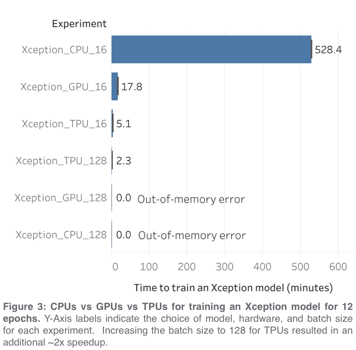
When to use CPUs vs GPUs vs TPUs in a Kaggle Competition. by Paul Mooney
In order to compare the performance of CPUs vs GPUs vs TPUs for accomplishing common data science tasks, we used the tf_flowers dataset to train a convolutional neural network, and then the exact same code was run three times using the three different backends (CPUs vs GPUs vs TPUs; GPUs were NVIDIA P100 with IntelXeon 2GHz (2 core) CPU and 13GB RAM. TPUs were TPUv3 (8 core) with IntelXeon 2GHz (4 core) CPU and 16GB RAM). The accompanying tutorial notebook demonstrates a few best practices for getting the best performance out of your TPU.
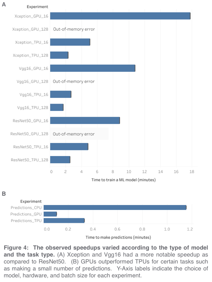
For our first experiment, we used the same code (a modified version*** of the official tutorial notebook) for all three hardware types, which required using a very small batch size of 16 in order to avoid out-of-memory errors from the CPU and GPU. Under these conditions, we observed that TPUs were responsible for a ~100x speedup as compared to CPUs and a ~3.5x speedup as compared to GPUs when training an Xception model (Figure 3). Because TPUs operate more efficiently with large batch sizes, we also tried increasing the batch size to 128 and this resulted in an additional ~2x speedup for TPUs and out-of-memory errors for GPUs and CPUs. Under these conditions, the TPU was able to train an Xception model more than 7x as fast as the GPU from the previous experiment****.
1位の方の記事をみると、まず、progressive pseudo-labelingという手法が気になった。類似コンペのデータをtrainingに使うのだが、つぎ足しながらtrainingするようである。CNNのモデルは、大きいほど良いらしく、DenseNet201まで使い、動かすのがたいへんらしい。Cutmix, ArcFaceLoss, Linear Sum Assignmentなど聞いたことのない単語がでてきてついていけない。
augmentation: flipping, rotating, scaling, color alterations (hue, saturation, brightness, and constrast), alterations in the H&E color space, additive noise, and Gaussian blurring.
1.上記のregularrizationやりすぎのような結果になった理由がわかったような気がする。A. Geronさんのテキスト341ページに次の記述がある。Finally, like a gift that keeps on giving, Batch Normalization acts like a regularizer, reducing the need for other regularization techniques (such as dropout, described later in this chapter).
関連する内容は、Using a pretrained convnetで始まり、feature extractionとfine-tuningという表現になっていて、transfer learningという用語は、少なくとも見出しには使われていない。全体がTransfer learningで、バリエーションが多いという感じがする。
4.NIPS 2019の論文
Transfusion: Understanding Transfer Learning for Medical Imaging Maithra Raghu∗ Cornell University and Google Brain maithrar@gmail.com Chiyuan Zhang∗ Google Brain chiyuan@google.com Jon Kleinberg† Cornell University kleinber@cs.cornell.edu Samy Bengio† Google Brain bengio@google.com Abstract Transfer learning from natural image datasets, particularly IMAGENET, using standard large models and corresponding pretrained weights has become a de-facto method for deep learning applications to medical imaging. However, there are fundamental differences in data sizes, features and task specifications between natural image classification and the target medical tasks, and there is little understanding of the effects of transfer. In this paper, we explore properties of transfer learning for medical imaging. A performance evaluation on two large scale medical imaging tasks shows that surprisingly, transfer offers little benefit to performance, and simple, lightweight models can perform comparably to IMAGENET architectures. Investigating the learned representations and features, we find that some of the differences from transfer learning are due to the over-parametrization of standard models rather than sophisticated feature reuse. We isolate where useful feature reuse occurs, and outline the implications for more efficient model exploration. We also explore feature independent benefits of transfer arising from weight scalings.
Automated Gleason Grading and Gleason Pattern Region Segmentation Based on Deep Learning for Pathological Images of Prostate Cancer. YUCHUN LI et al., IEEE Acsess 2020
Deep Isometric Learning for Visual Recognition Haozhi Qi, Chong You, Xiaolong Wang, Yi Ma, and Jitendra Malik arXiv:2006.16992v1 [cs.CV] 30 Jun 2020 Abstract Initialization, normalization, and skip connections are believed to be three indispensable techniques for training very deep convolutional neural networks and obtaining state-of-the-art performance. This paper shows that deep vanilla ConvNets without normalization nor skip connections can also be trained to achieve surprisingly good performance on standard image recognition benchmarks. This is achieved by enforcing the convolution kernels to be near isometric during initialization and training, as well as by using a variant of ReLU that is shifted towards being isometric. Further experiments show that if combined with skip connections, such near isometric networks can achieve performances on par with (for ImageNet) and better than (for COCO) the standard ResNet, even without normalization at all. Our code is available at https://github.com/HaozhiQi/ISONet.
Table 5
Since R-ISONet is prone to overfitting due to the lack of BatchNorm, we add dropout layer right before the finalclassifier and report the results in Table 5 (g). The results show that R-ISONet is comparable to ResNet with dropout (Table 5 (b)) and is better than Fixup with Mixup regularization (Zhang et al., 2018).
A subclass of ConnectionError, raised when trying to write on a pipe while the other end has been closed, or trying to write on a socket which has been shutdown for writing. Corresponds to errnoEPIPE and ESHUTDOWN.
A. Geronさんのテキストでは、AlexNetの説明のところで、Augmentationが紹介されている。AlexNetはoverfittingを防ぐためのgenerarization techniqueとして、DropoutとともにAugmentationを用いていたことが紹介されている。
F. Cholletさんのテキストでは、データが無限にあればoverfitは起きない。その代替方法として、データをランダムに加工することによって本物に近いデータを増やす方法としてAugmentationを位置づけている。さらに、data augmentationは、所詮、元画像の単純な加工に過ぎずoverfitthingを防ぐには十分でない。その場合には分類器の全結合層の手前にdropout(0.5)を入れるとよい、と説明されている。
さらに、コードの説明のところで、validation dataに対しては、Note that the validation data shouldn't be augmentedと書かれている。
しかし、Test Time Augmentationは、適切に用いれば大きな効果を発揮する可能性があるようだ。次のような論文がある。
Greedy Policy Search:A Simple Baseline for Learnable Test-Time Augmentation
Dmitry Molchanov, Alexander Lyzhov, Yuliya Molchanova, Arsenii Ashukha, and Dmitry Vetrov, arXiv:2002.09103v2 [stat.ML] 20 Jun 2020
Test-time data augmentation—averaging the predictions of a machine learning model across multiple augmented samples of data—is a widely used technique that improves the predictive performance. While many advanced learnable data augmentation techniques have emerged in recent years, they are focused on the training phase. Such techniques are not necessarily optimal for test-time augmentation and can be outperformed by a policy consisting of simple crops and flips. The primary goal of this paper is to demonstrate that test time augmentation policies can be successfully learned too. We introduce greedy policy search (GPS), a simple but high-performing method for learning a policy of test-time augmentation. We demonstrate that augmentation policies learned with GPS achieve superior predictive performance on image classification problems, provide better in-domain uncertainty estimation, and improve the robustness to domain shift.
Protein structure prediction using multiple deep neural networks in the 13th Critical Assessment of ProteinStructure Prediction (CASP13)
Andrew W. Senior1 | Richard Evans1 | John Jumper1 | James Kirkpatrick1 | Laurent Sifre1 | Tim Green1 | Chongli Qin1 | Augustin Žídek1 | Alexander W. R. Nelson1 | Alex Bridgland1 | Hugo Penedones1 | Stig Petersen1 | Karen Simonyan1 | Steve Crossan1 | Pushmeet Kohli1 | David T. Jones 2,3 | David Silver1 | Koray Kavukcuoglu1 | Demis Hassabis1 1 DeepMind, London, UK 2 The Francis Crick Institute, London, UK 3 University College London, London, UK
Abstract We describe AlphaFold, the protein structure prediction system that was entered by the group A7D in CASP13.
Submissions were made by three free-modeling (FM) methods which combine the predictions of three neural networks.
All three systems were guided by predictions of distances between pairs of residues produced by a neural network.
Two systems assembled fragments produced by a generative neural network, one using scores from a network trained to regress GDT_TS.
The third system shows that simple gradient descent on a properly constructed potential is able to perform on par with more expensive traditional search techniques and without requiring domain segmentation.
In the CASP13 FM assessors' ranking by summed z-scores, this system scored highest with 68.3 vs 48.2 for the next closest group (an average GDT_TS of 61.4).
The system produced high accuracy structures (with GDT_TS scores of 70 or higher) for 11 out of 43 FM domains.
Despite not explicitly using template information, the results in the template category were comparable to the best performing template-based methods.
KEYWORDS : CASP, deep learning, machine learning, protein structure prediction
AlphaFold at CASP13 Mohammed AlQuraishi 1,2,* 1Department of Systems Biology and 2Lab of Systems Pharmacology, Harvard Medical School, Boston, MA 02115, USA
Abstract Summary: Computational prediction of protein structure from sequence is broadly viewed as a foundational problem of biochemistry and one of the most difficult challenges in bioinformatics. Once every two years the Critical Assessment of protein Structure Prediction (CASP) experiments are held to assess the state of the art in the field in a blind fashion, by presenting predictor groups with protein sequences whose structures have been solved but have not yet been made publicly available.
The first CASP was organized in 1994, and the latest, CASP13, took place last December, when for the first time the industrial laboratory DeepMind entered the competition.
DeepMind’s entry, AlphaFold, placed first in the Free Modeling (FM) category, which assesses methods on their ability to predict novel protein folds (the Zhang group placed first in the Template-Based Modeling (TBM) category, which assess methods on predicting proteins whose folds are related to ones already in the Protein Data Bank.)
DeepMind’s success generated significant public interest.
Their approach builds on two ideas developed in the academic community during the preceding decade:
(i) the use of co-evolutionary analysis to map residue co-variation in protein sequence to physical contact in protein structure, and
(ii) the application of deep neural networks to robustly identify patterns in protein sequence and co-evolutionary couplings and convert them into contact maps.
In this Letter, we contextualize the significance of DeepMind’s entry within the broader history of CASP, relate AlphaFold’s methodological advances to prior work, and speculate on the future of this important problem.
1 Significance
Progress in Free Modeling (FM) prediction in Critical Assessment of protain Structure Prediction (CASP) has historically ebbed and flowed, with a 10-year period of relative stagnation finally broken by the advances seen at CASP11 and 12, which were driven by the advent of co-evolution methods (Moult et al., 2016, 2018; Ovchinnikov et ak., 2016; Schaarschumidt et al., 2018; Zhang et al., 2018) and the application of deep convolutional neural networks (Wang et al., 2017).
The progress at CAPS13 corresponds to roughly twice the recent rate of advance [measured in mean ΔGDT_TS from CASP10 to CASP12 - GDT_TS is a measure of prediction accuracy ranging from 0 to 100, with 100 being perfect (Zemla et al., 1999)].
This can be observed not only in the CASP-over-CASP improvement, but also in the gap between AlphaFold and the second best performer at CASP13, which is unusually large by CASP standards (Fig. 1).
Even when excluding AlphaFold, CASP13 shows further progress due to the widespread adoption of deep learning and the continued exploitation of co-evolutionary information in protain structure prediction (de Oliveira and Deane, 2017).
Taken together these obsevations indicate substantial progress both by the whole field and by AlphaFold in particular.
Nonetheless, the problem remains far from solved, particularly for practical applications.
GDT_TS measures gross topology, which is of inherent biological interest, but does not necessarily result in structures useful in drug discovery or molecular biology applications.
An alternative metric, GDT_HA, provides a more stringent assessment of atructural accuracy (Read and Chavali, 2017).
Figure 2 plots the GDT_HA scores of the top two performers for the last four CASPs.
While substantial progress can be discerned, the distance to perfect predictions remains sizeable.
In addition, both metrics measure global goodness of fit, which can mask significant local deviations.
Local accuracy corresponding to, for example, the coordination of atoms in an active site or the localized change of conformation due to a mutation, can be the most important aspect of a predicted structure when answering broader biological questions.
It remains the case however that AlphaFold represents an anomalous leap in protain structure prediction and portends favorably for the future.
In particular, if the AlphaFold-adjusted trend in Figure 1 were continue, then it is conceivable that in ~5 years' time we will begin to expect predicted structures with a mean GDT_TS of ~85%, which would arguably correspond to a solution of the gross topology problem.
Whether the trend will continue remains to be seen.
The exponential increase in the number of sequenced protains virtually ensures that improvements will be had even without new methodological developments.
However, for the more general problem of predicting arbitrary protain structures from an individual amino acid sequence, including designed ones, new conceptual breakthroughs will almost certainly be required to obtain further progress.
2 Prior work
AlphaFold is a co-evolution-dependent method building on the groundwork laid by several researchgroupes over the preceding decade.
Co-evolution methods work by first constructing a multiple sequence alignment (MSA) of protains homologous to the protain of interest.
Such MSAs must be large, often comprising 10^5-10^6 sequences, and evolutionarily diverse (Tetchner et al., 2014).
The so-called evolutionary couplings are then extracted from the MSA by detecting residues that co-evolve, i.e. that have mutated over evolutionary timeframes in response to other mutations, thereby suggesting physical proximity in space.
The foundational methodology behind this approach was developed two decades ago (Lapedes et al., 1999), but was originally only validated in simulation as large protain sequence families were not yet available.
The first set of such approaches to be applied effectively to real protains came after the exponential increase in availability of protain sequences (Jones et al., 2012; Kamisetty et al., 2013; Marks et al., 2011; Weigt et al., 2009).
These approaches predicted binary contact matrices from MSAs, i.e. whether two residues are 'in contact' or not (typically defined as having Cβ atoms within <8 Å), and fed that information to geomettric constraint satisfaction methods such as CNS (Brunger et al., 1998) to fold the protain and obtain its 3D coordinates.
This first generation of methods was a significant breakthrough, and ushered in the new era of protain structure prediction.
An important if expected development was the coupling of binary contacts with more advanced folding pipelines, such as Rosetta (Leaver-Fay et al., 2011) and I-Tasser (Yang et al., 2015), which resulted in better accuracy and constituted the state of the art in the FM category until the beginning of CASP12.
The next major advance came from applying convolutional networks (LeCun et al., 2015) and deep residual networks (He et al., 2015; Srivastava et al., 2015) to integrate information globally across the entire matrix of raw evolutionary coupling to obtain more accurate contacts (Liu et al., 2018; Wang et al., 2017).
This led to some of the advances seen at CASP12, although ultimately the best performing group at CASP12 did not make extensive use of deep learning [convolutional neural networks made a significant impact on contact prediction at CASP12, but the leading method was not yet fully implemented to have an impact on structure prediction (Wang et al., 2017)].
During the lead uo to CASP13, one group published a modification to their method, RaptorX (Xu, 2018), that proved highly consequential.
As before, RaptorX takes MSAs as inputs, but instead of predicting binary contacts, it predicts discrete distances.
Specifically, RaptorX predicts probabilities over discretized spatial ranges (e.g. 10% probability for 4-4.5 Å), then uses the mean and variance of the predicted distribution to calculate lower and upper bounds for atom-atom distances.
These bounds are then fed to CNS to fold the protain.
RaptorX showed promise on a subset of CASP13 targets, with its seemingly simple change having a surprisingly large impact on prediction quality.
Its innovation also forms one of the key ingredients of AlphaFold's approach.
3 AlphaFold
Similar to RaptorX, AlphaFold predicts a distribution over discretized spatial ranges as its output (the details of the convolutional network architecture are different).
Unlike RaptorX, which only exploits the mean and variance of the predicted distribution, AlphaFold uses the entire distribution as a (protain-specific) statistical potential function (Sippl, 1990; Thomas and Dill, 1996) that is directly minimized to fold the protain.
The key idea of AlphaFold's approach is that a distribution over pairwise distances between residues corresponds to a potential that can be minimized after being turned into a continuous function.
DeepMind's team initially experimented with more complex approaches (personal communication), including fragment assembly (Rohl et al., 2004) using a generative variational autoencoder (Kingma and Welling, 2013).
Halfway through CASP13 however, the team discovered thtat simple and direct minimization of the predicted energy function, using gradient descent (L-BFGS) (Goodfellow et al., 2016; Nocedal, 1980), is suffucient to yield accurate structures.
There are important technical details.
The potential is not used as is, but is normalized using a learned 'reference state', Human-derived reference states are a key component of knowledge-based potentials such as DFIRE (Zhang et al., 2005), but the use of a learned reference state is an innovation.
This potential is coupled with traditional physics-based energy terms from Rosetta and the combined function is what is actually minimized.
The idea of predicting a protain-specific energy potential is also not new (Zhao and Xu, 2012; Zhu et al., 2018), but AlphaFold's implementation made it highly performant in the structure prediction context.
This is important as protain-specific potentials are not widely used.
Popular knowledge- and physics-based potentials are universal, in that they aspire to be applicable to all protains, and in principle should yield a protain's lowest energy conformation with sufficient sampling.
AlphaFold's protain-specific potentials on the other hand are entirely a consequence of a given protain's MSA.
AlphaFold effectively constructs a potential surface that is very smooth for a given protain family, and whose minimum closely matches that of the family's avarage native fold.
Beyond the above conceptual innovations, AlphaFold uses more sophisticated neural networks than what has been applied in protain structure prediction.
First, they are hundreds of layers deep, resulting in a much higher number of parameters than existing approaches (Liu et al., 2018; Wang et al., 2017).
Second, through the use of so-called dilated convolutions, which use non-contiguous receptive fields that span a larger spatial extent than traditional convolutions, AlphaFold's neural networks can model long-range interactions covering the entirety of the protain sequence.
Third, AlphaFold uses sophisticated computational tricks to reduce the memory and compute requirements for processing long protain sequences, enabling the resulting networks to be trained for longer.
While these ideas are not new in the deep learning field, they had not yet been applied to protain structure prediction.
Combined with DeepMind's expertise in searching a large hyperparameter space of neural network configurations, they likely contributed substantially to AlphaFold's strong performance.
4 Future prospects
Much of the recent progress in protain structure prediction, including AlphaFold, has come from the incorporation of co-evolutionary data, which are by construction defined on the protain family level.
For predicting the gross topology of a protain family, co-evolution-dependent approaches will likely show continued progress for the foreseeable future.
However, such approaches are limited when it comes to predicting structures for individual protain sequences, such as a mutated or de novo designed protain, as they are dependent on large MSAs to identify co-variation in residures.
Lacking a large constellation of homologous sequences, co-evolution-dependent methods perform poorly, and this was observed at CASP13 for some of the targets on which AlphaFold was tested (e.g. T0998).
Physics-based approaches, such as Rosetta and I-Tasser, are currentry the primary paradigm for tackling this broader class of problems.
The advent of learning suggests a broader rethinking of how the protain structure problem could be tackled, however, with a broad range of possible new approaches, including end-to-end differentiable model (AlQuraichi, 2019; Ingraham et al., 2018), semi-supervised approaches (Alley et al., 2019; Bepler and Berger, 2018; Yang et al., 2018) and generative approaches (Anand et al., 2018).
While not yet broadly competitive with the best co-evolution-dependent methods, such approaches can eschew co-evolutionary data to directly learn a mapping function from sequence to structure.
As these approaches continue to mature, and as physico-chemical priors get more directly integrated into the deep learning machinery, we expect that they will provide a complementary path forward for tackling protain structure prediction.
Review Deep learning methods in protein structure prediction Mirko Torrisi b, Gianluca Pollastri b, Quan Le a,⇑ a Centre for Applied Data Analytics Research, University College Dublin, Ireland b School of Computer Science, University College Dublin, Ireland
a b s t r a c t Protein Structure Prediction is a central topic in Structural Bioinformatics.
Since the ’60s statistical methods, followed by increasingly complex Machine Learning and recently Deep Learning methods, have been employed to predict protein structural information at various levels of detail.
In this review, we briefly introduce the problem of protein structure prediction and essential elements of Deep Learning (such as Convolutional Neural Networks, Recurrent Neural Networks and basic feed-forward Neural Networks they are founded on), after which we discuss the evolution of predictive methods for one dimensional and two-dimensional Protein Structure Annotations, from the simple statistical methods of the early days, to the computationally intensive highly-sophisticated Deep Learning algorithms of the last decade.
In the process, we review the growth of the databases these algorithms are based on, and how this has impacted our ability to leverage knowledge about evolution and co-evolution to achieve improved predictions.
We conclude this review outlining the current role of Deep Learning techniques within the wider pipelines to predict protein structures and trying to anticipate what challenges and opportunities may arise next. 2020 The Authors. Published by Elsevier B.V. on behalf of Research Network of Computational and Structural Biotechnology.
1. Introduction Proteins hold a unique position in Structural Bioinformatics.
In fact, the origins of the field itself can be traced to Max Perutz and John Kendrew’s pioneering work to determine the structure of globular proteins (which also led to the 1962 Nobel Prize in Chemistry) [1,2].
The ultimate goal of Structural Bioinformatics, when it comes to proteins, is to unearth the relationship between the residues forming a protein and its function, i.e., in essence, the relationship between genotype and phenotype.
The ability to disentangle this relationship can potentially be used to identify, or even design, proteins able to bind specific targets [3], catalyse novel reactions [4] or guide advances in biology, biotechnology and medicine [5], e.g. editing specific locations of the genome with CRISPR-Cas9 [6].
According to Anfinsen’s thermodynamic hypothesis, all the information that governs how proteins fold is contained in their respective primary sequences, i.e. the chains of amino acids (AA, also called residues) forming the proteins [7,8].
Anfinsen’s hypothesis led to the development of computer simulations to score protein conformations, and, thus, search through potential states looking for that with the lowest free energy, i.e. the native state [9,8].
The key issue with this energy-driven approach is the explosion of the conformational search space size as a function of a protein’s chain length.
A solution to this problem consists in the exploitation of simpler, typically coarser, abstractions to gradually guide the search, as proteins appear to fold locally and non-locally at the same time but incrementally forming more complex shapes [10].
A standard pipeline for Protein Structure Prediction envisages intermediate prediction steps where abstractions are inferred which are simpler than the full, detailed 3D structure, yet structurally informative - what we call Protein Structure Annotations (PSA) [11].
The most commonly adopted PSA are secondary structure, solvent accessibility and contact maps.
The former two are one-dimensional (1D) abstractions which describe the arrangement of the protein backbone, while the latter is a two dimensional (2D) projection of the protein tertiary structure in which any 2 AA in a protein are labelled by their spatial distance, quantised in some way (e.g. greater or smaller than a given distance threshold).
Several other PSA, e.g. torsion angles or contact density, and variations of the aforementioned ones, e.g. halfsphere exposure and distance maps, have been developed to describe protein structures [11].
Fig. 1 depicts a pipeline for the prediction of protein structure from the sequence in which the intermediate role of 1D and 2D PSA is highlighted.
It should be noted that protein intrinsic disorder [12–14] can be regarded as a further 1D PSA with an important structural and functional role [15], which has been predicted by Machine Learning and increasingly Deep Learning methods similar to those adopted for the prediction of other 1D PSA properties [16–22], sometimes alongside them [23].
However, given its role in protein structure prediction pipelines is less clear than for other PSA, we will not explicitly focus on disorder in this article and refer the reader to specialised reviews on disorder prediction, e.g. [24–26].
The slow but steady growth in the number of protein structures available at atomic resolution has led to the development of PSA predictors relying also on homology detection (‘‘template-based predictors”), i.e. predictors directly exploiting proteins of known structure (‘‘templates”) that are considered to be structurally similar based on sequence identity [27–30].
However, a majority PSA predictors are ‘‘ab initio”, that is, they do not rely on templates.
Ab-initio predictors leverage extensive evolutionary information searches at the sequence level, relying on ever-growing data banks of known sequences and constantly improving algorithms to detect similarity among them [31–33].
Fig. 2 shows the growth in the number of known structures in the Protein Data Bank (PDB) [34] and sequences in the Uniprot [35] - the difference in pace is evident, with an almost constant number of new structures having been added to the PDB each year for the last few years while the number of known sequences is growing close to exponentially.
1.2. Deep Learning Deep Learning [41] is a sub-field of Machine Learning based on artificial neural networks, which emphasises the use of multiple connected layers to transform inputs into features amenable to predict corresponding outputs.
Given a sufficiently large dataset of input–output pairs, a training algorithm can be used to automatically learn the mapping from inputs to outputs by tuning a set of parameters at each layer in the network.
While in many cases the elementary building blocks of a Deep Learning system are FFNN or similar elementary cells, these are combined into deep stacks using various patterns of connectivity.
This architectural flexibility allows Deep Learning models to be customised for any particular type of data. Deep Learning models can generally be trained on examples by back-propagation [36], which leads to efficient internal representations of the data being learned for a task.
This automatic feature learning largely removes the need to do manual feature engineering, a laborious and potentially error-prone process which involves expert domain knowledge and is required in other Machine Learning approaches.
However, Deep Learning models easily contain large numbers of internal parameters and are thus data-greedy - the most successful applications of Deep Learning to date have been in fields in which very large numbers of examples are available [41].
In the remainder of this section we summarise the main Deep Learning modules which are used in previous research in Protein Structure Prediction.
Convolutional Neural Networks (CNN) [42] are an architecture designed to process data which is organised with regular spatial dependency (like the tokens in a sequence or the pixels in animage).
A CNN layer takes advantage of this regularity by applying the same set of local convolutional filters across positions in the data, thus brings two advantages: it avoids the overfitting problem by having a very small number of weights to tune with respect to the input layer and the next layer dimensionality, and it is translation invariant.
A CNN module is usually composed of multiple consecutive CNN layers so that the nodes at later layers have larger receptive fields and can encode more complex features.
It should be noted that ‘‘windowed” FFNN discussed above can be regarded as a particular, shallow, version of CNN, although we will keep referring to them as FFNN in this review to follow the historical naming practice in the literature.
Recurrent Neural Networks (RNN) [43] are designed to learn global features from sequential data.
When processing an input sequence, a RNN module uses an internal state vector to summarise the information from the processed elements of the sequence: it has a parameterised sub-module which takes as inputs the previous internal state vector and the current input element of the sequence to produce the current internal state vector; the final state vector will summarise the whole input sequence.
Since the same function is applied repeatedly across the elements of a sequence, RNN modules easily suffer from the gradient vanishing or gradient explosion problem [44] when applying the back propagation algorithm to train them.
Gated recurrent neural network modules like Long Short Term Memory (LSTM) [45] or Gated Recurrent Unit (GRU) [46] are designed to alleviate these problems.
Bidirectional versions of RNNs (BRNN) are also possible [47] and particularly appropriate in PSA predictions, where data instances are not sequences in time but in space and propagation of contextual information in both directions is desirable.
Even though the depth of a Deep Learning model increases its expressiveness, increasing depth also makes it more difficult to optimise the network weights due to gradients vanishing or exploding.
In [48] Residual Networks have been proposed to solve these problems.
By adding a skip connection from one layer to the next one, a Residual Network is initialised to be near the identity function thus avoids large multiplicative interactions in the gradient flow.
Moreover, skip connections act as ‘‘shortcuts”, providing shorter input–output paths for the gradient to flow in otherwise deep networks.
2. Methods for 1D Protein Structural Annotations
First generation PSA predictors relied on statistical calculations of propensities of single AA towards structural conformations, usually secondary structures [49–52], which were then combined into actual predictions via hand-crafted rules.
While these methods predicted at better than chance accuracy, they were quite limited - especially on novel protein structures [53], with per-AA accuracies usually not exceeding 60%.
In a second generation of predictors [54], information from more than one AA at a time was fed to various methods, including FFNN to predict secondary structure [38,39], and least squares, i.e. a standard regression analysis, to predict hydrophobicity values [55].
This step change was made possible by the increasing number of resolved structures available.
These methods were somewhat more accurate than first generation ones, with secondary structure accuracies of 63–64% reported [38]. The third generation of PSA predictors has been characterised by the adoption of evolutionary information [56] in the form of alignments of multiple homologous sequences as input to the predictive systems, which are almost universally Machine Learning, or Deep Learning algorithms.
One of the early systems from this generation, PHD [56], arguably the first to predict secondary structure at over 70% accuracy, was implemented as two cascaded FFNN taking segments of 13 AA and 17 secondary structure predictions as inputs, containing 5,000–15,000 free tunable parameters, and trained by back-propagation.
Subsequent sources of improvement were more sensitive tools for mining evolutionary information such as PSI-BLAST [32] or HMMER [57], and the ever increasing nature of both the databases of available structures and sequences, with PSIPRED [58], based on a similar stack of FFNN to that used in PHD, albeit somewhat larger, achieving state of the art performances at the time of development, with sustained 76% secondary structure prediction accuracy.
Various Deep Learning algorithms have been routinely adopted for PSA prediction since the advent of the third generation of predictors [11], alongside more classic Machine Learning methods such as k-Nearest Neighbors [63,64], Linear Regression [65], Hidden Markov Models [66], Support Vector Machines (SVM) [67] and Support Vector Regression [68].
PHD, PSIPRED, and JPred [69] are among the first notable examples in which cascaded FFNN are used to predict 1D PSA, in particular secondary structure. DESTRUCT [70] expands on this approach by simultaneously predicting secondary structure and torsion angles by an initial FFNN, then having a filtering FFNN map first stage predictions into new predictions, and then iterating, with all copies of the filtering network sharing their internal parameters.
SPIDER2 [59] builds on this approach adding solvent accessibility to the set of features predicted and training an independent set of weights for each iteration. The entire set of PSA predicted is used, along with the input features of the first stage, to feed the second and third stage.
Each stage is composed of a windowbased (w = 17) 3-layered FFNN with 150 hidden units each [59].
SSpro is a secondary structure predictor based on a Bidirectional RNN architecture followed by a 1D CNN stage.
The architecture was shown to be able to identify the terminus of the protein sequence and was quite compact with only between 1400 and 2900 free parameters [47].
Subsequent versions of SSpro increased the size of the training datasets and networks [71].
Similar architectures have been implemented to predict solvent accessibility and contact density [72].
The latest version of SSpro adds a final refinement step based on a PSI-BLAST search of structurally similar proteins [30], i.e. is a template-based predictor.
A variant to plain BRNN-CNN architectures are stacks of Recurrent and Convolutional Neural Networks [73,27,74,31,75].
In these a first BRNN-CNN stage is followed by a second structurally similar stage fed with averages over segments of predictions from the first stage.
Porter, PaleAle, BrownAle and Porter+ (Brewery) are Deep Learning methods employing these architectures to predict secondary structure, solvent accessibility, contact density and torsionangles, respectively [60,11].
The latest version of Porter (v5) is composed by an ensemble of 7 models with 40,000–60,000 free parameters each, using multiple methods to mine evolutionary information [31,76].
The same architecture has also been trained on a combination of sequence and structural data [27,28], and in a cascaded approach similar to that of DESTRUCT and SPIDER2 in which multiple PSA are predicted at once and the prediction is iterated [77].
SPIDER3 [61] substitutes the FFNN architecture of SPIDER2 with a Bidirectional RNN with LSTM cells [45] followed by a FFNN, predicts 4 PSA at once, and iterates the prediction 4 times. Each of the 4 iterations of SPIDER3 is made of 256 LSTM cells per direction per layer, followed by 1024 and 512 hidden units per layer in the FFNN.
Adam optimiser and Dropout (with a ratio of 50%) [78] are used to train the over 1 million free parameters of the model. SPIDER2 and SPIDER3 are the only described methods which employ seven representative physio-chemical properties in input along with both HHblits and PSI-BLAST outputs.
2.2. Convolutional neural networks
RaptorX-Property is a collection of 1D PSA predictors released since 2010 and based on Conditional Neural Fields (CNF), i.e. Neural Networks possessing an output layer made of Conditional Random Fields (CRF) [79].
The most recent version of RaptorX Property is based on Deep Convolutional Neural Fields (DeepCNF), i.e. CNN with CRF output [80,23].
This version has 5 convolutional layers containing 100 hidden units with a window size of 11 each, i.e. roughly 500,000 free parameters (10 times and 100 times as many as Porter5 and PHD, respectively).
The latest version of RaptorX-Property depends on HHblits instead of PSI-BLAST for the evolutionary information fed to DeepCNF models [23].
NetSurfP-2.0 is a recently developed predictor which employs either HHblits or MMsEqs. 2 [76,81], depending on the number of sequences in input [62].
NetSurfP-2.0 is made of two CNN layers, consisting of 32 filters with 129 and 257 units, respectively, and two BRNN layers, consisting of 1024 LSTM cells per direction per layer.
NetSurfP-2.0 predicts secondary structure, solvent accessibility, torsion angles and structural disorder with a different fully connected layer per PSA.
In Fig. 3 we report a scatterplot of performances of secondary structure predictors vs. the year of their release.
Gradual, continuing improvements are evident from the plot, as well as the transition from statistical methods to classical Machine Learning and later Deep Learning methods.
A set of surveys of recent methods for the prediction of protein secondary structure can be found in [82–85] and a thorough comparative assessment of highthroughput predictors in [86].
3. Methods for 2D Protein Structural Annotations A typical pipeline to predict protein structure envisages a step in which 2D PSA of some nature are predicted [11].
In fact, most of the recent progress in Protein Structure Prediction has been driven by Deep Learning methods applied to the prediction of contact or distance maps [87,88].
Contact maps have been adopted to reconstruct the full threedimensional (3D) protein structure since the ’90s [89–91].
Although the 2D-3D reconstruction is known to be a NP-hard problem [92], heuristic methods have been devised to solve it approximately [89,93,94] and optimised for computational efficiency [90].
The robustness of these heuristic methods has been tested against noise in the contact map [95].
Distance maps and multi-class contact maps (i.e. maps in which distances are quantised into more than 2 states) typically lead to more accurate 3D structures than binary maps and tend to be more robust when random noise is introduced in the map [29,96].
Nonetheless, one contact every twelve residues may be sufficient to allow robust and accurate topology-level protein structure modeling [97].
Predicted contact maps can also be helpful to score and, thus, guide the search for 3D models [98].
One of the earliest examples of 2D PSA annotations are β sheet pairings, i.e. AA partners in parallel and anti-parallel β sheet conformations.
Machine/Deep Learning methods such as FFNN [99], BRNN [100] and multi-stage approaches [101] have been used since the late ’90s to predict whether any 2 residues are partners in a β sheet.
Similarly, disulphide bridges (formed by cysteine-cysteine residues) have been predicted by the Edmonds-Gabow algorithm and Monte Carlo simulation annealing [102], or hybrid solutions such as Hidden Markov Models and FFNN [103], and multi-stage FFNN, SVM and BRNN [104], alongside classic Machine Learning models such as SVM [105], pure Deep Learning models such as BRNN [106], and FFNN [107].
The prediction of a contact map’s principal eigenvector (using BRNN) is instead an example of 1D PSA used to infer 2D characteristics [108].
The predictions of b sheet pairings, disulphide bridges and principal eigenvectors have been prompted by the need for ‘‘easy-to-predict”, informative abstractions which can be used to guide the prediction of more complex 2D PSA such as contact or distance maps.
Ultimately, however, most interest in 2D PSA has been in the direct prediction of contact and distance maps as these contain most, if not all, the information necessary for the reconstruction of a protein’s tertiary structure [89,29,96], while being translation and rotation invariant [91] which is a desirable property for the target of Machine Learning and Deep Learning algorithms.
Early methods for contact map prediction typically focused on simple, binary maps, and relied on statistical features extracted from evolutionary information in the form of alignments of multiple sequences.
Features such as correlated mutations, sequence conservation, alignment stability and family size were inferred from multiple alignments and were shown to be informative for contact map prediction since the ’90s [109,110].
Early methods often relied on simple linear combinations of features, though FFNN [111] and other Machine Learning algorithms such as Self-Organizing Maps [112] and SVM [113] quickly followed.
3.1. Modern and deep learning methods for 2D PSA prediction
2D-BRNN [72,124] are an extension to the BRNN architecture used to predict 1D PSA.
These models, which are designed to process 2D maps of variable sizes, have 4 state vectors summarising information about the 4 cardinal corners of a map.
2D-BRNN have been applied to predict contact maps [72,124,108,125], multi-class contact maps [29], and distance maps [96].
Contact map predictions by 2D-BRNN have also been refined using cascaded FFNN [126].
Both ab initio and template-based predictors have been developed to predict maps (as well as 1D PSA) [29,96].
In particular, template-based contact and distance map predictors rely both on the sequence and structural information and, thus, are often better than ab initio predictors even when only dubious templates are available [29,96].
More recently, growing abundance of evolutionary information data and computational resources has led to substantial breakthroughs in contact map prediction [127].
More sophisticated statistical methods have been developed to calculate mutual information without the influence of entropy and phylogeny [128], co-evolution coupling [129], direct-coupling analysis (DCA) [130] and sparse inverse covariance estimation [131].
The evergrowing number of known sequences has led to the development of more optimised and, thus, faster tools [132] able to also run on GPU [133].
PSICOV [131], FreeContact [132] and CCMpred [133], which are notable results of this development, have allowed the exploitation of ever growing data banks and prompted a new wave of Deep Learning methods.
MetaPSICOV is a notable example of a Deep Learning method applied to PSICOV, FreeContact and CCMpred, as well as 1D features (such as predicted 1D PSA) [134].
MetaPSICOV is a twostage FFNN with one hidden layer with 55 units.
MetaPSICOV2, the following version, is a two-stage FFNN with two hidden layers with 160 units each and also a template-based predictor [114].
DeepCDpred is a multi-class contact map ab initio predictor which attempts to extend MetaPSICOV [115].
In particular, PSICOV is substituted with QUIC - a similarly accurate but significantly faster implementation of the sparse inverse covariance estimation - and the two-stage FFNN with an ensemble of 7 deeper FFNN (with 8 hidden layers) which are trained on different targets and, thus, result in a multi-class map predictor.
RaptorX-Contact is one of the first examples of contact map predictor based on a Residual CNN architecture [116].
RaptorXContact has been trained on CCMpred, mutual information, pairwise potential extraction and RaptorX-Property’s output, i.e. secondary structure and solvent accessibility predictions [23].
RaptorX-Contact uses filters of size 3 x 3 and 5 x 5, 60 hidden units per layer and a total of 60 convolutional layers.
DNCON2 is a two-stage CNN trained on a set of input features similar to MetaPSICOV [117].
The first stage is composed of an ensemble of 5 CNN trained on 5 different thresholds, which feeds a following refining stage of CNN. The first stage of DNCON2 can be seen as a multi-class contact map predictor.
DeepContact (also known as i_Fold1) aims to demonstrate the superiority of CNN over FFNN to predict contact maps [118].
DeepContact is a 9-layer Residual CNN with 32 filters of size 5 x 5 trained on the same set of features used by MetaPSICOV.
The outputs of the third, sixth and ninth layers are concatenated with the original input and fed to a last hidden layer to perform the final prediction.
DeepCov uses CNN to predict contact maps when limited evolutionary information is available [119].
In particular, DeepCov has been trained on a very limited set of input features: pair frequencies and covariance.
This is one of the first notable examples of 2D PSA predictors which entirely skips the prediction of 1D PSA in its pipeline.
PconsC4 is a CNN with limited input features to significantly speed-up prediction time [120].
In particular, PconsC4 uses predicted 1D PSA, the GaussDCA score, APC-corrected mutual information, normalised APC-corrected mutual information and crossentropy.
PconsC4 requires only a recent version of Python and a GCC compiler with no need for any further external programs and appears to be significantly faster (and more accurate) than MetaPSICOV [120,114].
SPOT-Contact has been inspired by RaptorX-Contact and extends it by adding a 2D-RNN stage downstream of a CNN stage [121].
SPOT-Contact is an ensemble of models based on 120 convolutional filters – half 3 x 3 and half 5 x 5 – followed by a 2D-BRNN with 800 units – 200 LSTM cells for each of the 4 directions – and a final hidden layer composed of 400 units.
Adam, a 50% dropout rate and layer normalization are among the Deep Learning techniques implemented to train this predictor.
CCMpred, mutual and direct-coupling information are used as inputs as well as the output of SPIDER3, i.e. predictions of solvent accessibility, half-Sphere exposures, torsion angles and secondary structure [61].
TripletRes [122] is a contact map predictor that ranked first in the Contact Predictions category of the latest edition of CASP, a bi-annual blind competition for Protein Structure Prediction [135].
TripletRes is composed of 4 CNN trained end-to-end.
More in detail, 3 coevolutionary inputs, i.e. the covariance matrix, precision matrix and coupling parameters of the Potts model, are fed to 3 different CNN which are then fused in a unique CNN downstream.
Each CNN is composed of 24 residual convolutional layers with a kernel of size 3 x 3 x 64.
The training of TripletRes required 4 GPUs running concurrently - using Adam and a 80% dropout rate.
TripletRes successfully identified and predicted both globally and locally multi-domain proteins following a divide et impera strategy.
AlphaFold [123] is a Protein Structure Prediction method that achieved the best performance in the Ab initio category of CASP13 [135].
Central to AlphaFold is a distance map predictor implemented as a very deep residual neural networks with 220 residual blocks processing a representation of dimensionality 64 x 64 x 128 – corresponding to input features calculated from two 64 amino acid fragments.
Each residual block has three layers including a 3 x 3 dilated convolutional layer – the blocks cycle through dilation of values 1, 2, 4, and 8.
In total the model has 21 millions parameters.
The network uses a combination of 1D and 2D inputs, including evolutionary profiles from different sources and co-evolution features.
Alongside a distance map in the form of a very finely-grained histogram of distances, AlphaFold predicts U and W angles for each residue which are used to create the initial predicted 3D structure.
The AlphaFold authors concluded that the depth of the model, its large crop size, the large training set of roughly 29,000 proteins, modern Deep Learning techniques, and the richness of information from the predicted histogram of distances helped AlphaFold achieve a high contact map prediction precision.
Constant improvements in contact and distance map predictions over the last few years have directly resulted in improved 3D predictions.
Fig. 4 reports the average quality of predictions submitted to the CASP competition for free modelling targets, i.e. proteins for which no suitable templates are available and predictions are therefore fully ab initio, between CASP9 (2010) and CASP13 (2018).
Improvements especially over the last two editions are largely to be attributed to improved map predictions [127,136].
Proteins fold spontaneously in 3D conformations based only on the information present in their residues [7].
Protein Structure predictors are systems able to extract from the protein sequence information constraining the set of possible local and global conformations and use this to guide the folding of the protein itself.
Deep Learning methods are successful at producing higher abstractions/representations while ignoring irrelevant variations of the input when sufficient amounts of data are provided to them[137].
Both characteristics together with the availability of rapidly growing protein databases increasingly make Deep Learning methods the preferred techniques to aid Protein Structure Prediction (see Tables 1 and 2).
The highly complex landscape of protein conformations make Protein Structural Annotations one of the main research topics of interest within Protein Structure Prediction[11].
In particular, 1D annotations have been a central topic since the ’60s [1,2] while the focus is progressively shifting towards more informative and complex 2D annotations such as contactmaps and distance maps.
This change of paradigm is mainly motivated by technological breakthroughs which result in continuous growth in computational power and protein sequences available thanks to next-generation sequencing and metagenomics [76,81].
Recent work on the prediction of 1D structural annotations [11,31,75,61], contact map prediction [117,122], and on overall structure prediction systems [123,138], emphasises the importance of more sophisticated pipelines to find and exploit evolutionary information from ever growing databases.
This is often achieved by running several tools to find multiple homologous sequences in parallel [32,76,81] and, increasingly, by deploying Machine/Deep Learning techniques to independently process the sequence before fusing their outputs into the final prediction.
The correlation between sequence alignment quality and accuracy of PSA predictors has been empirically demonstrated [139–141].
How to best gather and process homologous sequences is an active research topic, e.g. RawMSA is a suite of predictors which proposes to substitute the pre-processing of sequence alignments with an embedding step in order to learn a representation of protein sequences instead of pre-compressing homologous sequences into input features [142].
The same trend towards end-to-end systems has been attempted in the pipeline from processed homologous sequences to 3D structure, e.g. inNEMO [143], a differentiable simulator, and RGN (Recurrent Geometrical Network) [144], an end-to-end differentiable learning of protein structure.
However, state-of-the-art structure predictors are still typically composed of multiple intelligent systems.
The last mile of Protein Structure Prediction, i.e. the building, ranking and scoring of structural models, is also fertile ground for Machine Learning and Deep Learning methods [145,146].
E.g. MULTICOM exploits DNCON2 - a multi-class contact map predictor - to build structural models and to feed DeepRank - an ensemble of FFNN to rank such models [138].
DeepFragLib is, instead, a Deep Learning method to sample fragments (for ab initio structure prediction) [147].
The current need for multiple intelligent systems is supported by empirical results, especially in the case of hard predictions.
Splitting proteins into composing domains, predicting 1D PSA, and optimising each component of the pipeline is particularly useful especially when alignment quality is poor [148].
Today, state-of-the-art systems for Protein Structure Prediction are composed by multiple specialised components [123,138,11] in which Deep Learning systems have an increasing, often crucial role, while end-to-end prediction systems entirely based on Deep Learning techniques, e.g. Deep Reinforcement Learning, may be on the horizon but are at present still immature.
Progress in this field over the last few years has been substantial, even dramatic especially in the prediction of contact and distance maps [127,136], but the essential role of structural, evolutionary, and co-evolutionary information in this progress cannot be understated, with ab initio prediction quality still lagging that of template-based predictions, proteins with poor alignments being still a weak spot and prediction of protein structure from a single sequence being a challenge that is far from solved [149], although some progress has recently been observed for proteins with shallow alignments [150].
More generally, given that our current structure prediction pipelines rely almost exclusively on increasingly sophisticated and sensitive techniques to detect similarity to known structures and sequences, it is unclear whether predictions truly represent low energy structures unless we know they arecorrect.
The prediction of protein misfolding [151,152] presents a further challenge for the current prediction paradigm, with Machine Learning methods only making slow inroads [153].
Nevertheless, as more computational resources, novel techniques and ultimately, critically, increasing amounts of experimental data will become available [137], further improvements are to be expected.
Many domains of science have developed complex simulations to describe phenomena of interest.
While these simulations provide high-fidelity models, they are poorly suited for inference and lead to challenging inverse problems.
We review the rapidly developing field of simulation-based inference and identify the forces giving additional momentum to the field.
Finally, we describe how the frontier is expanding so that a broad audience can appreciate the profound influence these developments may have on science.
approximate Bayesian computation | neural density estimation
Mechanistic models can be used to predict how systems will behave in a variety of circumstances.
These run the gamut of distance scales, with notable examples including particle physics, molecular dynamics, protain folding, population genetics, neuroscience, epidemiology, economics, ecology, climate science, astrophysics, and cosmology.
The expressiveness of programming languages facilitates the development of complex, high-fidelity simulations and the power of modern computing provides the ability to generate synthetic data from them.
Unfortunately, these simulators are poorly suited for statistical inference.
The source of the challenge is that the probability density (or likelihood) for a given observation - an essential ingredient for both frequentist and Bayesian inference methods - is typically intractable.
Such models are often referred to as implicit models and contrasted against prescribed models where the likelihood for an observation can be explicitly calculated (1).
The problem setting of statistical inference under intractable likelihoodshas been dubbed likelihood-free inference - although it is a bit of a misnomer as typically one attempts to estimate the intractable likelihood, so we feel the term simulation-based inference is more apt.
推論手法は、ABCのように、推論中にシミュレーター自体を使用するものと、代理モデルを構築して推論に使用する方法に大きく分けることができます。最初のケースでは、シミュレーターの出力がデータと直接比較されます(図1 A–D)。後者の場合、シミュレーターの出力は、図1 E – Hの緑色のボックスに示すように、推定またはMLステージのトレーニングデータとして使用されます。結果の代理モデルは、赤い六角形で示され、推論に使用されます。