Chapter 8 Dimensionality Reduction
Hands-On Machine Learning with Scikit-Learn, Keras & Tensorflow 2nd Edition by A. Geron
Many Machine Learning problems involve thousands or even millions of features for each training instance.
Not only do all these features make training extremely slow, but they can also make it much harder to find a good solution, as we will see.
This problem is often refered to as the curse of dimentionality.
Fortunately, in real-world problems, it is often possible to reduce the number of features considerably, turning an intractable problem into a tractable one.
For example, consider the MNIST images (introduced in Chapter 3):
the pixels on the image borders are almost always white, so you could completely drop these pixels from the training set without losing much information.
Figure 7-6 confirms that these pixels are utterly unimportant for the classification task.
Additionally, two neighboring pixels are often highly correlated:
if you merge them into a single pixel (e.g., by taking the mean of the two pixel intensities), you will not lose much information.
振り返ると、手書き文字(数字)認識のMNISTは、toy problemにしか見えない。
Reducing dimensionality does cause some information loss (just like compressing an image to JPEG can degrade its quality), so even though it will speed up training, it may make your system perform slightly worse.
It also makes your pipeline a bit more complex and thus harder to maintain.
So, if training is too slow, you should first try to train your system with the original data before considering using dimensionality reduction.
In some cases, reducing the dimensionality of the training data may filter out some noise and unnecessary details and thus result in higher performance, but in general it won't:
it will just speed up training.
Apart from speeding up training, dimensionality reduction is also extremely useful for data visualization (or DataVis).
Reducing the number of dimensions down to two (or three) makes it possible to plot a condensed view of a high-dimensional training set on a graph and often gain some important insights by visually detecting patterns, such as clusters.
Moreover, DataViz is essential to communicate your conclusions to people who are not data scientists - in particular, decision makers who will use your results.
In this chapter we will discuss the curse of dimensionality and get a sense of what goes on in high-dimensional space.
Then, we will consider the two main approaches to dimensionality reduction (projection and Manifold Learning), and we will go through three of the most popular dimensionality reduction techniques:
PCA, Kernel PCA, and LLE.
The Curse of Dimensionality
We are so used to living in three dimensions that our intuition fails us when we try to imagine a high-dimensional space.
Even a basic 4D hypercube is incredibly hard to picture in our mind (see Figure 8-1), let alone a 200-dimensional ellipsoid bent in a 1,000-dimensional space.

It turns out that many things behave very differently in high-dimensional space.
For example, if you pick a random point in a unit square (a 1 x 1 square), it will have only about a 0.4% chance of being located less than 0.001 from a border (in other words, it is very unlikely that a random point will be "extreme" slong any dimension).
But in a 10,000-dimensional unit hypercube, this probability is greater than 99.000000%.
Most points in a high-dimensional hypercube are very close to the border.
*理解できない。
Here is a more troublesome difference:
if you pick two points randomly in a unit square, the distance between these two points will be, on average, roughly 0.52.
If you pick two random points in a unit 3D cube, the average distance will be roughly 0.66.
But what about two points picked randomely in a 1,000,000-dimensional hypercube?
The average distance, believe it or not, will be about 408.25 (roughly √1,000,000/6)!
This is counterintuitive:
how can two points be so far apart when they both lie within the same unit hypercube?
Well, there's just plenty of space in high dimensions.
As a result, high-dimensional datasets are at risk of being very sparse:
most training instances are likely to be far away from each other.
This also means that a new instance will likely be far away from any training instance, making predintions much less reliable than in lower dimensions, since they will be based on much larger extrapolations.
In short, the more dimensions the training set has, the greater the risk of overfitting it.
*理解できない。
In theory, one solution to the curse of dimensionality could be to increase the size of the training set to reach a sufficient density of training instances.
Unfortunately, in practice, the number of training instances required to reach a given density grows exponentially with the number of dimensions.
With just 100 features (significantly fewer than in the MNIST problem), you would need more instances than atoms in the observable universe in order for training instances to be within 0.1 of each other on average, assuming they were spread out uniformly across all dimensions.
*理解できない。
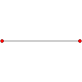


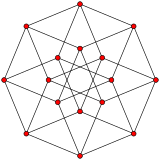


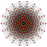
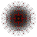
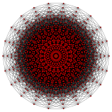
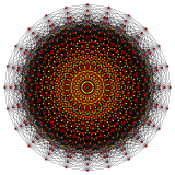
n-cube can be projected inside a regular 2n-gonal polygon by a skew orthogonal projection, shown here from the line segment to the 12-cube.
Hypercube:Wikipediaからの、12次元までの画像。
Main Approaches for Dimensionality Reduction


