Hands-On Machine Learning with Scikit-Learn, Keras & Tensorflow 2nd Edition by A. Geron
Many Machine Learning problems involve thousands or even millions of features for each training instance.
Not only do all these features make training extremely slow, but they can also make it much harder to find a good solution, as we will see.
This problem is often refered to as the curse of dimentionality.
Fortunately, in real-world problems, it is often possible to reduce the number of features considerably, turning an intractable problem into a tractable one.
For example, consider the MNIST images (introduced in Chapter 3):
the pixels on the image borders are almost always white, so you could completely drop these pixels from the training set without losing much information.
Figure 7-6 confirms that these pixels are utterly unimportant for the classification task.
Additionally, two neighboring pixels are often highly correlated:
if you merge them into a single pixel (e.g., by taking the mean of the two pixel intensities), you will not lose much information.
振り返ると、手書き文字(数字)認識のMNISTは、toy problemにしか見えない。
Reducing dimensionality does cause some information loss (just like compressing an image to JPEG can degrade its quality), so even though it will speed up training, it may make your system perform slightly worse.
It also makes your pipeline a bit more complex and thus harder to maintain.
So, if training is too slow, you should first try to train your system with the original data before considering using dimensionality reduction.
In some cases, reducing the dimensionality of the training data may filter out some noise and unnecessary details and thus result in higher performance, but in general it won't:
it will just speed up training.
Apart from speeding up training, dimensionality reduction is also extremely useful for data visualization (or DataVis).
Reducing the number of dimensions down to two (or three) makes it possible to plot a condensed view of a high-dimensional training set on a graph and often gain some important insights by visually detecting patterns, such as clusters.
Moreover, DataViz is essential to communicate your conclusions to people who are not data scientists - in particular, decision makers who will use your results.
In this chapter we will discuss the curse of dimensionality and get a sense of what goes on in high-dimensional space.
Then, we will consider the two main approaches to dimensionality reduction (projection and Manifold Learning), and we will go through three of the most popular dimensionality reduction techniques:
PCA, Kernel PCA, and LLE.
The Curse of Dimensionality
We are so used to living in three dimensions that our intuition fails us when we try to imagine a high-dimensional space.
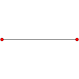
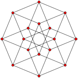
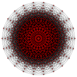
Even a basic 4D hypercube is incredibly hard to picture in our mind (see Figure 8-1), let alone a 200-dimensional ellipsoid bent in a 1,000-dimensional space.
Figure 8-1. Point, segment, square, cube, and tesseract (0D to 4D hypercubes) from Wikipedia
It turns out that many things behave very differently in high-dimensional space.
For example, if you pick a random point in a unit square (a 1 x 1 square), it will have only about a 0.4% chance of being located less than 0.001 from a border (in other words, it is very unlikely that a random point will be "extreme" slong any dimension).
But in a 10,000-dimensional unit hypercube, this probability is greater than 99.000000%.
Most points in a high-dimensional hypercube are very close to the border.
*理解できない。
Here is a more troublesome difference:
if you pick two points randomly in a unit square, the distance between these two points will be, on average, roughly 0.52.
If you pick two random points in a unit 3D cube, the average distance will be roughly 0.66.
But what about two points picked randomely in a 1,000,000-dimensional hypercube?
The average distance, believe it or not, will be about 408.25 (roughly √1,000,000/6)!
This is counterintuitive:
how can two points be so far apart when they both lie within the same unit hypercube?
Well, there's just plenty of space in high dimensions.
As a result, high-dimensional datasets are at risk of being very sparse:
most training instances are likely to be far away from each other.
This also means that a new instance will likely be far away from any training instance, making predintions much less reliable than in lower dimensions, since they will be based on much larger extrapolations.
In short, the more dimensions the training set has, the greater the risk of overfitting it.
*理解できない。
In theory, one solution to the curse of dimensionality could be to increase the size of the training set to reach a sufficient density of training instances.
Unfortunately, in practice, the number of training instances required to reach a given density grows exponentially with the number of dimensions.
With just 100 features (significantly fewer than in the MNIST problem), you would need more instances than atoms in the observable universe in order for training instances to be within 0.1 of each other on average, assuming they were spread out uniformly across all dimensions.
*理解できない。
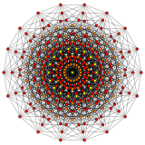
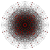
n-cube can be projected inside a regular 2n-gonal polygon by a skew orthogonal projection, shown here from the line segment to the 12-cube.
Hands-On Machine Learning with Scikit-Learn, Keras & Tensorflow 2nd Edition by A. Geron
Suppose you pose a complex question to thousands of random people, then aggregate their answers. In many cases you will find that thisaggregated answer is better than an expert's answer. This is called the wisdom of crowd.
Similaely, if you aggregate the predictions of a group of predictors (such as classifiers or regressors), you will often get better predictions than with the best indivisual predictor.
A group of predictors is called an ensemble; thus this technique is called Ensemble Learning, and an Ensemble Learning algorithm is called an Ensemble method.
As an example of an Ensemble method, you can train a grope of Decision Tree classifiers, each on a different random subset of the training set.
To make predictions, you obtain the predictions of all the individual trees, then predict the class that gets the most votes (see the last exercise in Chapter 6).
Such an ensemble of Decision Trees is called a Random Forest, and despite its simplicity, this is one of the most powerful Machine Learning algorithms available today.
As discussed in Chapter 2, you will often use Ensemble methods near the end of a project, once you have already built a few good predictors, to combine them into an even better predictor. In fact, the winning solutions in Machine Learning competitions often involve several Ensemble methods.
In this chapter we will discuss the most popular Ensemble methods, including bagging, boosting, and atacking. We will also explore Random Forests.
Voting Classifiers
Suppose you have trained a few classifiers, each one achieving about 80% accuracy.
You may have a Logistic Regression classifier, an SVM classifier, a Random Forest Classifier, a K-Nearest Neighbors classifier, and perhaps a few more.
A very simple way to create an even better classifier is to aggregate the predictions of each classifier and predict the class that gets the most votes.
This majority-vote classifier is called a hard voting classifier.
Somewhat surprisingly, this voting classifier often achieves a higher accuracy than the best classifier in the ensemble.
In fact, even if each classifier is a weak learner (meaning it does only slightly better than random guessing), the ensemble can still be a strong learner (achieving high accuracy), provided there are a sufficient number of weak learners and they are sufficiently diverse.
*Ensembleが良い結果をもたらす理由の1つは、generalization、にありそうだな。
Ensemble methods work best when the predictors are as independent from one another as possible.
One way to get diverse classifiers is to train them using very different algorithm.
This increases the chance that they will make very different types of errors, improving the ensemble's accuracy.
The following code creates and trains a voting classifier in Scikit-Learn, composed of three diverse classifiers (the training set is the moons dataset, introduced in Chapter 5):
from sklearn.ensemble import RandomForestClassifier
from sklearn.ensemble import VotingClassifier
from sklearn.linear_model import LogisticRegression
The voting classifier slightly outperforms all the individual classifiers.
If all classifiers are able to estimate class probabilities (i.e., they all have a predict_proba( ) method), then you can tell Scikit-Learn to predict the class with the highest class probability, averaged over all the individual classifiers.
This is called soft voting.
It often achieves higher performance than hard voting because it gives more weight to highly confident votes.
All you need to do is replace voting="hard" with voting="soft" and ensure that all classifiers can estimate class probabilities.
This is not the case for the SVC class by default, so you need to set its probability hyperparameter to True (this will make the SVC class use cross-validation to estimate class probabilities, slowing down training, and it will add a predict_proba( ) method).
If you modify the preceding code to use soft voting, you will find that the voting classification achieves over 91.2% accuracy!
Hands-On Machine Learning with Scikit-Learn, Keras & Tensorflow 2nd Edition by A. Geron
Like SVMs Decision Trees are versatile Machine Learning algorithms that can perform both classification and regression tasks, and even multioutput tasks.
They are powerful algorithms, capable of fitting complex datasets.
For example, in Chapter 2 you trained a DecisionTreeRegressor model on the California housing dataset, fitting it perfectly (actually, overfitting it).
Decision Trees are also the fundamental components of Random Forests (see Chapter 7), which are among the most powerful Machine Learning algorithms available today.
In this chapter we will start by discussing how to train, visualize, and make predictions with Decision Trees.
Then we will go through the CART training algorithm used by Scikit-Learn, and we will discuss how to regularrize trees and use them for regression tasks.
Finally, we will discuss some of the limitations of Decision Trees.
Training and Visualizing a Decision Tree
To understand Decision Trees, let's build one and take a look at how it makes predictions.
The following code trains a DecisionTreeClassifier on the iris dataset (see Chapter 4):
from sklearn.datasets import load_iris
from sklearn.tree import DecisionTreeClassifier
iris = load_iris( )
X = iris.data[ : , 2: ] # petal length and width
y = iris.target
tree_clf = DecisionTreeClassifier(max_depth=2)
tree_clf.fit(X, y)
Figure 6-1. Iris Decision Treeは表示できないので省略。
Making Predictions
Let's see how the tree represented in Figure 6-1 makes predictions.
Suppose you find an iris flower and you want to classify it.
You start at the root node (depth 0, at the top):
this node asks whether the flower's petal length is smaller than 2.45 cm.
If it is, then you move down to the root's left child node (depth 1, left).
In this case, it is a leaf node (i.e., it does not have any child nodes), so it doed not ask any questions:
simply look at the predicted class for that node, and the Decision Tree predicts that your flower is an Iris setosa (class=setosa).
Now suppose you find another flower, and this time the petal length is greater than 2.45 cm.
You must move down to the root's right child node (depth 1, right), which is not a leaf node, so the node asks another question:
is the petal width smaller than 1.75 cm?
If it is, then your flower is most likely an Iris versicolor (depth 2, left).
If not, it is likely an Iris virginica (depth 2, right).
It's really that simple.
One of the many qualities of Decision Trees is that they require very little data preparation.
In fact, they don't require feature scaling or centering at all.
Hands-On Machine Learning with Scikit-Learn, Keras & Tensorflow 2nd Edition by A. Geron
A Support Vector Machine (SVM) is a powerful and versatile Machine Learning model, capable of performing linear or nonlinear classification, regression, and even outlier detection.
It is one of the most popular models in Machine Learning, and anyone interested in Machine Learning should have it in their toolbox.
SVMs are particularly well suited for classification of complex small- or medium-sized datasets.
This Chapter will explain the core concepts of SVMs, how to use them, and how they work.
The fundamental idea behind SVMs is best explained with some pictures.
Figure 5-1 shows part of the iris dataset that was introduced at the end of Chapter 4.
The two classes can clearly be separated easily with a straight line (they are linearly separable).
The left plot shows the decision boundaries of three possible linear classifiers.
The model whose decision boundary is represented by the dashed line is so bad that it does not even separate the classes properly.
The other two models work perfectry on this training set, but their decision boundaries come so close to the instances that these models will probably not perform as well on new instances.
In contrast, the solid line in the plot on the right represent the decision boundaries of an SVM classifier;
this line not only separates the two classes but also stays as far away from the closest training instanses as possible.
You can think of an SVM classifier as fitting the widest possible street (represented by the parallel dashed lines) between the classes.
This is called large margin classification.
Figure 5-1. Large margin classification
Notice that adding more training instances "off the street" will not affect the decision boundary at all:
it is fully determined (or "supported") by the instances located on the edge of the street.
These instances are called the support vectors (they are circled in Figure 5-1).
SVMs are sensitive to the feature scale, as you can see in Figure 5-2:
in the left plot, the vertical scale is much larger than the horizontal scale, so the widest possible street is close to horizontal.
After feature scaling (e.g., using Scikit-Learn's StandardScaler), the decision boundary in the right plot looks much better.
Figure 5-2. Sensitivity to feature scale
Soft Margin Classification
If we strictly impose that all instances must be off the street and on the right side, this is called hard margin classification.
There are two main issues with hard margin classification.
First, it only works if the data is linearly separable.
Second, it is sensitive to outliers.
Figure 5-3 shows the iris dataset with just one additional outlier:
on the left, it is impossible to find a hard margin;
on the right, the decision boundary ends up very different from the one we saw in Figure 5-1 without the outlier, and it will probably not generalize as well.
Figure 5-3. Hard margin sensitivity to outliers
To avoid these issues, use a more flexible model.
The objective is to find a good balance between keeping the street as large as possible and limiting the margin violations (i.e., instances that end up in the middle of the street or even on the wrong side).
This is called soft margin classification.
When creating an SVM model using Scikit-Learn, we can specify a number of hyperparameters.
C is one of those hyperparameters.
If we set it to a low value, then we end up with the model on the left of Figure 5-4.
However, in this case the model on the left has a lot of margin violations but will probably generalize better.
Figure 5-4. Large margin (left) versus fewer margin violations (right)
If your SVM model is overfitting, you can try regularlizing it by reducing C.
The following Scikit-Learn code loads the iris dataset, scale the features, and then trains a linear SVM model (using the linear SVC class with C=1 and the hinge loss function, described shortly) to detect Iris virginica flowers.
Unlike Logistic Regression classifiers, SVM classifiers do not output probabilities for each class.
Instesd of using the Linear SVC class, we could use the SVC class with a linear kernel.
When creating the SVC model, we would write SVC(kernel="linear", C=1).
Or we could use the SGDClassifier class, with SGDClassifier(loss="hinge", alpha=1/(m*C)).
This applies regular Stochastic Gradient Descent (see Chapter 4) to train a linear SVM classifier.
It does not converge as fast as the Linear SVC class, but it can be useful to handle online classification tasks or huge datasets that do not fit in memory (out-of-core training).
The LinearSVC class regularizes the bias term, so you should center the training set first by subtracting its mean.
This is automatic if you scale the data using the StandardScaler.
Also make sure you set the loss hyperparameter to "hinge", as it is not the default value.
Finally, for better performance, you should set the duel hyperparameter to False, unless there are more features than training instances (we will discuss duality later in the chapter).
The LinearRegression class is based on the scipy.linalg.lstsq( ) functions (the name stands for "linear squares"), which you could call directry:
theta_best_svd, residuals, rank, s = np.linalg.lstsq(X_b, y, rcond=1e-6)
theta_best_svd
array([[4.21509616],
[2.77011339]])
You can use np.linalg.pinv( ) to compute the pseudoinverse directly.
np.linalg.pinv(X_b).dot(y)
array([[4.21509616],
[2.77011339]])
最後に、seudoinverseの計算方法、Singular Value Decomposition (SVD):特異値分解を用いる方法について説明している。
SVDは、残念ながら、フォローできない。
Computational Complexity
前節に引き続き、計算方法について説明しているようである。
Gradient Descent
Gradient Descentは、wide range of problemsに対して、optimal solution を見つけることができるgeneric optimization algolismである。general idea of Gradient Descentは、cost functionをminimizeするためにparameterをiterativeにtwak(微調整)することである。
Figure 4-10. The first 20 steps of Stochastic Gradient Descent
Mini-batch Gradient Descent
Figure 4-11. Gradient Descent paths in parameter space
polynomial Regression
What if your data is more complex than a stright line?
Surprisingly, you can use a linear model to fit nonlinear data.
A simple way to do this is to add powers of each feature as new features, then train a linear model on this extended set of features.
This technique is called Polynomial Regression.
Let's look at an example.
First, let's generate somo nonlinear data, based on a simple quadratic equation (plus some noise; see figure 4-12):
m = 100
X = 6 * np.random.rand(m, 1) - 3
y = 0.5 * X**2 + X + 2 + np.random.randn(m, 1)
Clearly, a straight line will never fit this data property.
So let's use Scikit-Learn's PolynomialFeatures class to transform our training data, adding the square (second-degree polynomial) of each feature in the training set as a new feature (in this case there is just one feature):
from sklearn.preprocessing import PolynomialFeatures
Not bad: the model estimates y-hat = 0.56*x1^2 + 0.93*x1 + 1.78 when in fact the original function was y = 0.5*x1^2 + 1.0*x1 +2.0 + Gaussian noise.
Note that when there are multiple features, Polynomial Regression is capable of finding relationships between features (which is something a plain Linear Regression model cannot do).
This made possible by the fact that PolynomialFeatures also adds all combinations of features up to the given degree.
For example, if there were two features a and b, PolynomialFeatures with degree=3 would not only add the features a^2, a^3, b^2, and b^3 but also the combinations ab, a^2b, and ab^2.
PolynomialFeatures (degree=d) transforms an array containing n features into an array containing (n + d)!/d!n! features, where n! is the factorial of n, 1 x 2 x 3 x ... x n.
Beware of the combinatorial explosion of the number of features!
def fetch_spam_data(spam_url=SPAM_URL, spam_path=SPAM_PATH): if not os.path.isdir(spam_path): os.makedirs(spam_path) for filename, url in *2: path = os.path.join(spam_path, filename) if not os.path.isfile(path): urllib.request.urlretrieve(url, path) tar_bz2_file = tarfile.open(path) tar_bz2_file.extractall(path=SPAM_PATH) tar_bz2_file.close()
HAM_DIR = os.path.join(SPAM_PATH, "easy_ham") SPAM_DIR = os.path.join(SPAM_PATH, "spam") ham_filenames = [name for name in sorted(os.listdir(HAM_DIR)) if len(name) > 20] spam_filenames = [name for name in sorted(os.listdir(SPAM_DIR)) if len(name) > 20]
We ca use Python's email module to parse these emails (this handles headers, encoding, and so on):
import email import email.policy
def load_email(is_spam, filename, spam_path=SPAM_PATH): directory = "spam" if is_spam else "easy_ham" with open(os.path.join(spam_path, directory, filename), "rb") as f: return email.parser.BytesParser(policy=email.policy.default).parse(f)
ham_emails = [load_email(is_spam=False, filename=name) for name in ham_filenames] spam_emails = [load_email(is_spam=True, filename=name) for name in spam_filenames]
Let's look at one example of ham and one example of spam, to get a feel of what the data looks like:
Some emails are actually multipart, with images and attachiments (which can have their own attachments). Let's look at the various types of structures we have.
It seems that the ham emails are more often plain text, while spam has quite a lot of HTML. Moreover, quite a few ham emails are sighned using PGP , while no spam is. In short, it seems that the email structure is useful information to have.
Okay, let's start writing the preprocessing functions. First, we will need a function to convert HTML to plain text. Arguably the best way to do this would be to use the great BeautifulSoupe library, but I would like to avoid adding another dependency to this project, so let's hack a quick & dirty solution using regular expressions.
The following function first drops the <head> section, then converts all <a> tags to the word HYPERLINK, then it gets rid of all HTML tags, leaving only the plain text. For readability, it also replaces multiple newlines with single newlines, and finally it unescapes html entities (such as > or ):
import re
from html import unescape
def html_to_plain_text(html):
text = re.sub('<head.*?>.*?</head>', '', html, flags=re.M | re.S | re.I)
OTC Newsletter Discover Tomorrow's Winners For Immediate Release Cal-Bay (Stock Symbol: CBYI) Watch for analyst "Strong Buy Recommendations" and several advisory newsletters picking CBYI. CBYI has filed to be traded on the OTCBB, share prices historically INCREASE when companies get listed on this larger trading exchange. CBYI is trading around 25 cents and should skyrocket to $2.66 - $3.25 a share in the near future. Put CBYI on your watch list, acquire a position TODAY. REASONS TO INVEST IN CBYI A profitable company and is on track to beat ALL earnings estimates! One of the FASTEST growing distributors in environmental & safety equipment instruments. Excellent management team, several EXCLUSIVE contracts. IMPRESSIVE client list including the U.S. Air Force, Anheuser-Busch, Chevron Refining and Mitsubishi Heavy Industries, GE-Energy & Environmental Research. RAPIDLY GROWING INDUSTRY Industry revenues exceed $900 million, estimates indicate that there could be as much as $25 billi ...