この1か月間でmachine learning, deep learingの燃料電池開発への応用について学ぶ。
Fundamentals, materials, and machine learning of polymer electrolyte membrane fuel cell technology
Yun Wang et al., Energy and AI 1 (2020) 100014
Machine learning and artificial intelligence (AI) have received increasing attention in material/energy development. This review also discusses their applications and potential in the development of fundamental knowledge and correlations, material selection and improvement, cell design and optimization, system control, power management, and monitoring of operation health for PEM fuel cells, along with main physics in PEM fuel cells for physics-informed machine learning.
4. Machine learning in PEMFC development
4.1. Machine learning overview
According to learning style, machine learning algorithms can be generally classified into three types: supervised learning(教師あり学習), unsupervised learning(教師なし学習), and reinforcement learning(強化学習), as shown in Table 9 .

Table 10 lists popular supervised learning algorithms and their characteristics.

Among many machine learning(機械学習) methods, the rapid development of deep learning(ディープラーニング) in recent years has pushed it to the forefront of the field of AI.
Deep learning is the ANN with deep structures or multi-hidden layers [229-232] .
It can achieve good performance with the support of big data and complex physics, and has a much simpler mathematical form than many traditional machine learning algorithms.
(分子や結晶の構成原子の3次元原子座標と原子番号から、第一原理計算結果によってエネルギーや電子分布やエネルギーバンド計算などを行い、構成原子の3次元座標と原子番号と、第一原理計算結果を教師データにして、ANNを学習させると、新たに構成原子の3次元座標と原子番号を、学習させたANNに入力すれば、エネルギーや電子分布やエネルギーバンド計算結果が、第一原理計算を行ったのと同等の正確さで、ANNから出力することができる。)
The relationship between AI, machine learning, and deep learning is shown in Fig. 2 , along with the number of US patent applications per year [20] .
We can expect that deep learning, such as physics-informed learning, will become the most important path to AI.
(画像分類や自然言語処理などに用いられるANNは、教師データによってゼロから学ぶことによって分類や翻訳の機能を習得するのだが、自然科学分野への応用においては、ANNに物理化学の基礎を追加することによって、ANNは物理化学の分野において、大型計算機を使った場合と同等以上の正確さで、かつ、非常に短時間で、結果を出力できるようになってきている。)
However, deep learning relies on big data, and thus traditional machine learning still have strong applications, especially for interdisciplinary studies, and can solve problems with reasonable amounts of data.
Many open-source machine learning frameworks have been developed and made available to the general public, including Scikit-Learn, Caffe2, H2O, PyTorch (for neural networks), TensorFlow (for neural networks), and Keras (for neural networks).
4.2. Machine learning for performance prediction
PEMFC performance is characterized by the polarization curve, also called the I-V curve, which is determined by a number of factors including fuel cell dimensions, material properties, operation conditions, and electrochemical/physical processes [233-236] .
Various physical models and experimental methods have been proposed to predict or di- rectly measure the I-V curve, which are reviewed by many other works [ 158 , 160 , 202 , 237 ].
As an alternative approach, machine learning is capable of establishing the relationship between inputs and output performance through proper training of existing data, as shown in Fig. 18 .

Mehrpooya et al. [233] experimentally constructed a database of PEMFC performance under various inlet humidity, temperature, and oxygen and hydrogen flow rates.
A two-hidden-layer ANN was then trained using the database to predict the performance under new conditions.
Total 460 points are contained in the database with 400 for training and 60 for testing, and R 2 of 0.982 (for the training) and 0.9723 (for the test) was achieved in their study.
(このレベルの内容では、手間がかかる割には、効果は少ない(小さい)と思う。)
Unlike physical models, the mapping between inputs and outputs constructed by machine learning models does not follow an actual physical process; thus, the machine learning approach is also called the blackbox model.
Machine learning has unique advantages in PEMFC modeling, which requires no prior knowledge, especially of the complex coupled transport and electrochemical processes occurring in PEMFC operation.
This significantly reduces the level of modeling difficulty and also makes it possible to take into account any processes in which the physical mechanisms are not yet known or formulated.
The machine learning method is also advantageous in terms of computational efficiency in the implementation process after proper training.
This characteristic makes machine learning potentially extremely important in the practical PEMFC applications which usually involve a large size multiple-cell system, dynamic variation, and long-term operation.
For a complex physical model that takes multi-physics into account, the computational and time costs are usually too high; a simplified physical model lacks of high prediction accuracy.
For even a small scale stack of 5–10 cells, physics model-based 3D simulation usually requires 10–100 million gridpoints and takes days or weeks for predicting one case of steady-state operation [ 158 , 160 , 241 ].
In this regard, machine learning could greatly help to broaden the application of complex physical models by leveraging on prediction accuracy and computational efficiency.
Using the simulation data from complex physical models to train a machine learning model is a popular approach, usually referred to as surrogate modeling.
A surrogate model can replace the complex physical model with similar prediction accuracy but higher computational efficiency.
Wang et al. [242] developed a 3D fuel cell model with a CL agglomerate sub-model to construct a database of the PEMFC performance with various CL compositions.
A data-driven surrogate model based on the SVM was then trained using the database, which exhibited comparable prediction capability to the original physical model with several-order higher computational efficiency.
It only took a second to predict an I-V curve using the surrogate model versus hundreds of processor-hours using the 3D physics-based model.
Owing to its computational efficiency of the surrogate model, the surrogate model, coupled with a generic algorithm (GA), is suitable for CL composition optimization.
Similarly, Khajeh-Hosseini-Dalasm et al. [243] combined a CL physical model and ANN to develop a surrogate model to predict the cathode CL performance and activation overpotential.
For fast prediction of the multi-physics state of PEM fuel cell, Wang et al. [244] developed a data-driven digital twinning frame work, as shown in Fig. 20 .
A database of temperature, gas reactant, and water content fields in a PEM fuel cell under various operating conditions was constructed using a 3D physical model.
Both ANN and SVM were used to solve the multi-physics data with spatial distribution characteristics.
The data-driven digital twinning framework mirrored the distribution characteristics of multi-physics fields, and ANN and SVM exhibited different prediction performances on different physics fields.
There is a great potential to improve the current two-phase models (e.g. the two-fluid and mixture approaches) of PEM fuel cells by using AI technology, for example, machine learning analysis of visualization data and VOF/LBM simulation results.
可視化データの機械学習分析やVOF / LBMシミュレーション結果などのAIテクノロジーを使用することで、PEM燃料電池の現在の2相モデル(2流体および混合アプローチなど)を改善する大きな可能性がある。
Physics-informed neural networks were recently proposed by Raissi et al. [174] , known as hidden fluid mechanics (HFM), to encode the Navier-Stokes (NS) equation into deep learning for analyzing fluid flow images, as shown in Fig. 21 .
Raissiらは、Navier-Stokesの式をディープラーニングに組み込むことによって、流体の流れを可視化することを可能にした、物理情報(この場合はNavier-Stokesの式)に基づくニューラルネットワーク、hidden fluid mechanics (HFM)、を最近提案した。
Such a strategy can be extended to the deep learning of two-phase flow and fuel cell performance by incorporating relevant physics, such as the capillary pressure correlation, Darcy’s law, and the Butler-Volmer equation, into the neural networks.
このような戦略は、キャピラリー圧力相関、ダルシーの法則、バトラー・ボルマー方程式などの関連する物理学をニューラルネットワークに組み込むことにより、二層流と燃料電池の性能の深層学習に拡張できます。
Table 11 summarizes the main physics in each PEMFC component that deep learning can incorporate to effec- tively achieve the design targets.
表11は、ディープラーニングが設計目標を効果的に達成するために組み込むことができる各PEMFCコンポーネントの主な物理学をまとめたものです。

4.3. Machine learning for material selection
Machine learning is widely used in the chemistry and material communities to discover new material properties and develop next generation materials [245-247] .
Experimental measurement, characterization and theoretical calculation are main traditional methods to diagnose or predict the properties of a material, which are usually expensive in terms of cost, time, and computational resources.
Material properties are influenced by many intricate factors, which increases the difficulty level in the search for optimal material synthesis using only traditional methods.
Machine learning can assist in material selection and property prediction using existing databases, which is advantageous in taking into account unknown physics and greatly increasing the efficiency.
As example, in the catalyst design absorbate binding energy prediction by the empirical Sabatier principle is widely used for the optimization of activity in catalyst design ( Fig. 22 (a)) [247] .
To remove the empirical equation, a database of binding energy for different catalyst structures constructed by characterization or theoretical calculation is used to train a machine learning model, which shows a great efficiency in predicting the catalyst activity in a wide range to identify the optimal solution of the catalyst structure ( Fig. 22 (b)).
Owing to the great potentials of machine learning in chemistry and materials science, professional tools have been developed, along with universal machine learning frameworks, and numerous structure and property databases for molecules and solids can be easily accessed to model training.
Popular professional machine learning tools and databases are summarized in Table 12.
4.4. Machine learning for durability
A durable and stable PEM fuel cell that is reliable for the entire life of the system is crucial for its commercialization.
Thus, it is important to predict the state of health (SoH), the remaining useful life (RUL), and durability of PEM fuel cell using the data generated from monitoring units.
The cell voltage is the most important indicator of fuel cell performance and thus is a popular output parameter in the machine learning.
In recent years, machine learning has been employed to predict fuel cell durability and SoH, which can generally be classified as model-based and data-driven approaches.
fuel cell + materials informaticsとfuel cell + deep learningでGoogle Scholarで検索した。
+ matrials informaticsでは、2020年以降の論文のタイトルに、materials informaticsが入っている論文は2件しか出てこなかった。どちらも著者は日本人である。
+ deep learningでは、10件以上あり、machine learningやreinforcement learningなども含めると30件くらいは出てくる。
自分の直観では、materials informaticsは探索手段の1つにmachine learningやdeep learningを取り込み、それにによってパワーアップされた結果、machine learningやdeep learningなどが、materials informaticsの主要部分として牽引しているように思う。
7月18日(日)

表1(a)には、4種類の燃料電池の出荷量の推移が示され、(b)にはPEMFC(polymer electrolyte membrane fuel cell)固体高分子形燃料電池の構成/構造図が示されている。
DMFC : Direct Methanol Fuel Cell, SOFC : Solid Oxide Fuel Cell, PAFC : Phospholic Acid Fuel Cell, PEMFC : Polymer Electrolyte Membrane Fuel Cell
セルの中央に高分子電解質膜、その左側にアノード触媒、右側にカソード触媒、さらに左側には水素の拡散層、右側には空気(酸素源)の拡散層がある。カソードの最外層を冷媒が流れる。アノード側で気体水素が水素イオンと電子に、カソード側で水素イオンと酸素と電子が水に変化する。
1.2. Current status and technical barriers
PEMFCの課題は、耐久性とコスト。
触媒層のコストとセルの耐久性は相反する。
1.3. Role of fundamentals, materials, and machine learning
7月20日(火)
4.2. Machine learning for performance prediction
引用文献[174]を見てみよう。
Hidden fluid mechanics: Learning velocity and pressure fields from flow visualizations
Maziar Raissi, Alireza Yazdani, and George Em Karniadakis, Science 367, 1026–1030 (2020)
For centuries, flow visualization has been the art of making fluid motion visible in physical and biological systems. Although such flow patterns can be, in principle, described by the Navier-Stokes equations, extracting the velocity and pressure fields directly from the images is challenging. We addressed this problem by developing hidden fluid mechanics (HFM), a physics-informed deep-learning framework capable of encoding the Navier-Stokes equations into the neural networks while being agnostic to
the geometry or the initial and boundary conditions. We demonstrate HFM for several physical and biomedical problems by extracting quantitative information for which direct measurements may not be possible. HFM is robust to low resolution and substantial noise in the observation data, which is important for potential applications.
何世紀にもわたって、流れの可視化は、物理的および生物学的システムで流体の動きを可視化する技術でした。 このような流れのパターンは、原則としてナビエ・ストークス方程式で表すことができますが、画像から直接速度場と圧力場を抽出することは困難です。 この問題に対処するために、物理学に基づいた深層学習フレームワークである隠れ流体力学(HFM)を開発しました。これは、ジオメトリや初期条件や境界条件に依存せずに、ナビエ-ストークス方程式をニューラルネットワークにエンコードできます。 直接測定が不可能な可能性のある定量的情報を抽出することにより、いくつかの物理的および生物医学的問題に対するHFMを示します。 HFMは、観測データの低解像度とかなりのノイズに対してロバストです。これは、潜在的なアプリケーションにとって重要です。by Google翻訳

We developed an alternative approach, which we call hidden fluid mechanics (HFM), that simultaneously exploits the information available in snapshots of flow visualizations and the NS equations, combined in the context of physicsinformed deep learning (5) by using automatic differentiation. In mathematics, statistics, and computer science—in particular, in machine learning and inverse problems—regularization is the process of adding information in order to prevent overfitting or to solve an ill-posed problem. The prior knowledge of the NS equations introduces important structure that effectively regularizes the minimization procedure in the training of neural networks. For example, using several snapshots of concentration fields (inspired by the drawings of da Vinci in Fig. 1A), we obtained quantitatively the velocity and pressure fields (Fig. 1, B to D).
自動微分を使用して、流れの可視化とNS方程式のスナップショットで利用可能な情報を、物理情報に基づく深層学習(5)のコンテキストで組み合わせて同時に活用する、隠れ流体力学(HFM)と呼ばれる代替アプローチを開発しました。 数学、統計学、コンピューターサイエンス、特に機械学習と逆問題では、正則化とは、過剰適合を防止したり、不適切な問題を解決したりするために情報を追加するプロセスです。 NS方程式の予備知識は、ニューラルネットワークのトレーニングにおける最小化手順を効果的に正規化する重要な構造を導入します。 たとえば、濃度場のいくつかのスナップショット(図1Aのダヴィンチの図に触発された)を使用して、速度場と圧力場を定量的に取得しました(図1、BからD)。by Gppgle翻訳
7月28日(水)
基礎知識:
ムーアの新物理化学:W. J. MOORE著 藤代亮一訳:
8章 化学反応速度論
37.活性化吸着
吸着が起こるまでに乗り越さねばならないポテンシャルエネルギーの障壁はしばしば小さいかまたは無視される程度であるから、吸着の速度は裸の表面に気体の送り込まれる速さによって支配される。しかしながら、吸着にかなりの活性化エネルギーEadを必要とする場合があり、そのときの吸着速度(A*exp(-Ead/RT)は充分小さくなって表面反応の全体の速度がこれによって決定されるようになるだろう。このようにかなりの活性化エネルギーを要する吸着は活性化吸着とよばれる。
一般に金属表面上の気体の化学吸着にはあまり活性化エネルギーを必要とはしない。J. K. Robertsは、注意してきれいにした金属線上への水素の吸着は約25°Kでさえも速やかに進行し、強く水素原子の吸着された単分子層(単原子層)を作ることを示した。このときの吸着熱は、金属の水素化物の共有結合を作るのに要する熱量に近い。
・・・これと異なる挙動を示す一つの重要な例外は400℃における鉄触媒上への窒素の吸着である。この吸着はおそい活性化吸着で、この触媒を用いるアンモニア合成反応の律速段階であるように思われる。・・・
38.触媒の被毒
触媒はごく少量の異物によって被毒作用をうける。Faradayは、H2とO2の結合反応の触媒として用いる白金は、きれいで脂のついていないもので、また反応気体は一酸化炭素を含んでいてはならないと強調した。SO2をSO3に酸化する白金の非常に有効な触媒作用については19世紀の初めによく知られていたが、触媒がすぐにその活性を失うため、興行的には用いられなかった。高度に純粋にした反応気体、すなわち、イオウとヒ素化合物を除いた反応気体が得られて初めて長時間にわたって反応を続けさせることができた。
CO、H2S、ヒ素化合物のような触媒毒が強い生理学的毒物でもあることは、偶然の一致ではない。これらが動物に毒作用を呈する理由は、生存に必要な生化学反応を促進する酵素の被毒によって、その生化学反応が禁止されるからである。
触媒毒と反応物は有効な触媒表面のとり合いをする。・・・。ここで触媒の失活の程度は、毒によって占められた表面の割合と定量的に対応するだろうかという重要な疑問が生ずる。これはある場合には正しいが、少量の毒によってその表面積効果だけからは説明できないほど大きな阻害を受ける場合もよく知られている。
39.触媒表面の性質
巨視的には滑らかな固体表面でも10Åの単位では凹凸がある。最も優れた光学的技術によってへき開した結晶面を調べると、それが階段状の表面であることがわかる。金属からの光電子放射や熱イオン放射の実験を行うと、表面はいろいろ異なった仕事関数をもった部分からできていることがわかる。・・・。また結晶の稜や角、粒子と粒子の境界その他表面の物理的な不規則性は、異常に高い触媒作用をもつ活性中心になると考えられる。
7月29日(木)
元の論文に戻ろう。
Fundamentals, materials, and machine learning of polymer electrolyte membrane fuel cell technology, Yun Wang et al., Energy and AI 1 (2020) 100014

Hydrogen Oxydation Reaction (HOR) :
アノード触媒層中では、水素ガス(水素分子)が酸化(電子を失う)され、水素イオン(H+)と電子が生じる。
HORによって発生した水素イオン(H+)は、高分子電解質(Polymer Electrolyte Material:PEM)層中を移動し、カソード触媒層中に移動する。
Oxygen Reduction Reaction (ORR) :
カソード触媒層中では、酸素ガス(酸素分子)が水素イオン(H+)によって還元(電子を得る、水素と化合する)され、水(H2O)を生じる。
上図の左側から順に、水素ガス拡散層、アノード触媒層、高分子電解質層、カソード触媒層、酸素ガス拡散層、が積層されている。
3. Fundamentals and materials
For the hydrogen oxidation reaction (HOR) and oxygen reduction reaction (ORR) to proceed efficiently, the materials used in fuel cells must be chosen so that a high beginning of life performance and durability are ensured.
For example, to improve the activation and reduce transport losses, various issues as discussed earlier need to be addressed, including durable electrocatalyst and its loading reduction [2] , reactant/membrane contamination [ 91 , 92 ], water management [ 93 , 94 ], and degradation [ 95 , 96 ].
Material advance and improvement are therefore important for fuel cell R&D, and fundamentals that establish the material properties and fuel cell performance under various operation conditions are highly needed.
3.1. Materials
3.1.1. Membrane
The PEM is located between the anode and cathode CLs.
Its main functions are two-fold:
(i) it acts as a separator between the anode and the cathode reactant gasses and electrons, and
(ii) it conducts protons from the anode to cathode CLs.
Therefore, as a separator it must be impermeable to gasses (i.e., it should not allow the crossover of hydrogen and oxygen) and must be electrically insulating.
In addition, the membrane material must withstand the harsh operating conditions of PEM fuel cells, and thus possess high chemical and mechanical stability [97] .


これは、Nafion XLのSEM像
8月4日(水)
3.1.2. Catalyst layers
Catalyst layers (CLs) are the component where the electrochemical reactions occur.
触媒層は、電気化学反応が生じる場である。
The CL material must provide continuous pathways for various reactant species; primarily,
(i) a path for proton transport,
水素イオンの移動
(ii) a pore network for gaseous reactant supply and water removal, and
水素ガスと酸素ガスの供給、水の排出
(iii) a passage for electron conduction between the CL and the current collector.
触媒層と集電体層の間の電子(電荷)の移動
The CL material is a major factor affecting fuel cell performance and durability.
Conventional CLs are composed of electrocatalyst, carbon support, ionomer, and void space.
従来型の触媒層は、電極触媒、炭素支持体、アイオノマー、及び、空隙からなる。
Optimization of the CL ink preparation has been the main driver in PEMFC development [ 21 , 102 ].
This breakthrough highlights the importance of the so-called triple-phase boundaries of the ionomer, Pt/C, and void space so that all reactants could access for the reactions.
Conventional CLs are prepared based on the dispersion of a catalyst ink comprising a Pt/C catalyst, ionomer, and solvent.
従来型の触媒層は、Pt/C触媒とアイオノマーと溶媒からなる触媒インクの分散(体)をベースに調整(調製)される。
Ink composition is important for aggregation of the ionomer and agglomeration of carbon particles, and the dispersion medium governs the ink’s properties, such as the aggregation dimension of the catalyst/ionomer particles, viscosity, and rate of solidification, and ultimately, the electrochemical and transport properties of the CLs [103-105] .
The ionomer not only acts as a binder for the Pt/C particles but also proton conductor.
アイオノマーは、Pt/Cのバインダーとしてだけでなくプロトン導電体としての機能も有する
Imbalance in the ionomer loading increases the transport or ohmic loss, with a small amount of ionomer reducing the proton conductivity and a large amount increasing the transport resistance of gaseous reactants.
アイオノマーが少ないと、イオン電導性が下がり、アイオノマーが多いと、(空隙率が下がるため)、気体反応物の輸送特性が低下する。
8月5日(木)
Understanding inks for porous-electrode formation
Kelsey B. Hatzell, Marm B. Dixit, Sarah A. Berlinger and Adam Z. Weber J. Mater. Chem. A, 5, 20527 (2017)
Scalable manufacturing of high-aspect-ratio multi-material electrodes are important for advanced energy storage and conversion systems. Such technologies often rely on solution-based processing methods where the active material is dispersed in a colloidal ink. To date, ink formulation has primarily focused on macro-scale process-specific optimization (i.e. viscosity and surface/interfacial tension), and been optimized mainly empirically. Thus, there is a further need to understand nano- and mesoscale interactions and how they can be engineered for controlled macroscale properties and structures related to performance, durability, and material utilization in electrochemical systems.
高アスペクト比のマルチマテリアル電極のスケーラブルな製造は、高度なエネルギー貯蔵および変換システムにとって重要です。 このような技術は、多くの場合、活物質がコロイドインクに分散される溶液ベースの処理方法に依存しています。 これまで、インクの配合は主にマクロスケールのプロセス固有の最適化(つまり、粘度と表面/界面張力)に焦点を当てており、主に経験的に最適化されてきました。 したがって、ナノスケールとメソスケールの相互作用、および電気化学システムの性能、耐久性、材料利用に関連する制御されたマクロスケールの特性と構造のためにそれらをどのように設計できるかをさらに理解する必要があります。by Google翻訳


In summary, there is a growing need for fabricating porous electrodes with unprecedented control of layer composition. Key to this is knowledge of the underlying physics and phenomena going from multicomponent dispersions and inks to casting/processing to 3D structure. While there has been some recent work as highlighted herein, a great deal remains to be accomplished in order to inform predictive and not empirical optimizations. Such investigations have occurred in other fields such as semiconductors and coatings and dispersions in general, but this has not been translated to thin-film properties and functional layers as occur in electrochemical devices. Overall, ink engineering is an exciting opportunity to achieve next-generation composite materials, but requires systematic studies to elucidate design rules and metrics and identify controlling parameters and phenomena.
要約すると、層組成の前例のない制御を備えた多孔質電極を製造する必要性が高まっている。これの鍵は、多成分分散液やインクからキャスティング/プロセッシング、3D構造に至るまでの基礎となる物理学と現象に関する知識です。ここで強調されているように最近の作業がいくつかありますが、経験的な最適化ではなく予測的な最適化を通知するために、多くのことを達成する必要があります。このような調査は、一般に半導体やコーティング、分散液などの他の分野で行われていますが、これは電気化学デバイスで行われるような薄膜特性や機能層には変換されていません。全体として、インクエンジニアリングは次世代の複合材料を実現するための刺激的な機会ですが、設計ルールと測定基準を解明し、制御パラメーターと現象を特定するための体系的な研究が必要です。by google翻訳
元の論文に戻ろう。
Fundamentals, materials, and machine learning of polymer electrolyte membrane fuel cell technology, Yun Wang et al., Energy and AI 1 (2020) 100014
In contrast, non-conventional CLs are structured such that one of the major ingredients in their conventional counterparts is eliminated [ 2 , 102 ].
Nanostructured thin film (NSTF) CLs from 3 M are the most successful nonconventional CL.
They consist of whiskers where the catalyst is deposited without ionomer for proton conduction.
Over the years, they have proven to provide a higher activity than conventional CLs, as seen in Fig. 5 .
In addition, similar to conventional CLs, annealing can be used to change the CL structure and ultimately change its activity.

Fig. 5. Schematic illustration and corresponding HRTEM images of the mesoscale ordering during annealing and formation of the mesostructured thin film starting from the as-deposited Pt–Ni on whiskers (A), annealed at 300 °C (B) and 400 °C (C). Specific activities of Pt–Ni NSTF as compared to those of polycrystalline Pt and Pt-NSTF at 0.9 V (D) [106] .
[106] van der Vliet DF , Wang C , Tripkovic D , et al. Mesostructured thin films as electrocatalysts with tunable composition and surface morphology. Nat Mater 2012;11:1051–8 .
8月10日(火):ペースアップ
Carbon is the most commonly used support material for catalyst because of its low cost, chemical stability, high surface area, and affinity for metallic nanoparticles.
The surface area of the support varies depending on its graphitization process and is reported to range from 10 to 2000 m 2 /g [107] .
Ketjen Black and Vulcan XC-72 are popular carbons with a surface area of 890 m 2 /g and 228 m 2 /g, respectively [108] .
Carbon tends to aggregate, forming carbon particle agglomerates with a bimodal pore size distribution (PSD).
This PSD is usually composed of the primary pores of typically 2–20 nm in size and sec- ondary pores larger than 20 nm.
The primary pores are located between carbon particles in an agglomerate, while the secondary pores are between agglomerates.
Depending on the Pt distribution and utilization within an agglomerate, the primary pores play a key role in determining the electrochemical kinetics, while the secondary pores are important for reactant transport across a CL.
The portion of the primary and secondary pores is largely determined by the surface area of the carbon support [108] .
Hence, it has been reported that carbon supports also determine the optimal ionomer content and the Pt distribution in CLs [ 109 , 110 ].
Additionally, the anode overpotential is usually considered negligible in comparison with its cathode counterpart because of the sluggish ORR.
Thus, most work in the literature is focused on cathode CLs.
CL optimization is focused on not only enhanced durability but also reduction of the Pt loading.
For this purpose, it is crucial to determine the optimal combination of the carbon support and catalyst for loading reduction.
An example is highlighted in Fig. 6 , where different carbons are heat-treated to induce the catalytic activities of PANI- derived catalysts and to ensure their performance and stability.
Rotating Ring-Disk Electrode (RDE) measurements were conducted to study the ORR activity of various heat-treated PANI-C catalysts as a function of temperature.

The durability and stability of CL material are a major subject in R&D, which is related to multiple factors, mainly including (i) operating and environmental conditions, (ii) oxidant and fuel impurities, and (iii) contaminants and corrosion in cell components.
For instance, operation under high voltages (above 1.35 V), which may occur during fuel cell startup and shut-down, can lead to Pt dissolution [112] .
Operation further above this voltage will cause degradation of the carbon support, known as carbon corrosion.
In addition, any traces of a contaminant in the fuel or oxidant feeds can lead to a decrease in fuel cell performance by poisoning CL materials [ 113 , 114 ].
Some contaminants cover the Pt catalyst and then reduce the electrochemical surface area (ECSA) available for the reaction.
This catalytic contamination is usually reversible upon removal of the contaminants.
In certain instances, contaminants such as ammonia will cause irreversible degradation under adequate exposure time and concentration [44] .
Further, cell components, such as CLs and BPs, may contain contaminants, from their manufacturing process and/or material used, which eventually leach out and cause poi- soning of the MEA.
This may include membrane poisoning by metallic cations [91] .
Up to date, Pt is the electrocatalyst of choice for the ORR in PEM fuel cells because of its high activity.
However, Pt has a high cost associated with it and is currently mined in mainly several countries, such as South Africa and Russia.
Furthermore, high Pt loading is required to reach the target lifetime without major efficiency loss.
Using state-of-the-art methods, Pt catalyst is distributed in a way that does not allow its full utilization in CLs [ 115 , 116 ].
Alternative catalysts that are either Pt free or Pt alloys are under research.
Two excellent review papers on the topic are provided by Ref. [ 117 , 118 ].
A summary of some of these catalysts, their current status, and remaining challenges is provided in Fig. 7 .

Machine learning and AI are extremely helpful and highly demanding for CL development providing that CLs have been extensively studied for not only PEM fuel cells, but also many other systems, such as electrolyzers and sensors with Pt-catalyst electrodes.
The species transport equations, ORR reaction kinetics, two-phase flow, and degrada- tion mechanisms can be encoded into the neural networks for effective physics-informed deep learning to understand the impacts of catalyst materials on fuel cell performance/durability and optimize the pore size, PSD, PTFE loading, ionomer content, and carbon and electrocatalyst loading.
In the mass production phase, machine learning and AI can assist the quality control of CL composition in signal processing and element analysis when integrated with detection techniques such as Laser Induced Breakdown Spectroscopy (LIBS) [119] .
文献検索:keyword : fuel cell deep learning
F.-K. Wang et al.: Hybrid Method for Remaining Useful Life Prediction of PEMFC Stack
ABSTRACT
Proton exchange membrane fuel cell (PEMFC) is a clean and efficient alternative technology for transport applications. The degradation analysis of the PEFMC stack plays a vital role in electric vehicles. We propose a hybrid method based on a deep neural network model, which uses the Monte Carlo dropout approach called MC-DNN and a sparse autoencoder model to analyze the power degradation trend of the PEMFC stack. The sparse autoencoder can map high-dimensional data space to low-dimensional latent space and significantly reduce noise data. Under static and dynamic operating conditions, using two experimental PEMFC stack datasets the predictive performance of our proposed model is compared with some published models. The results show that the MC-DNN model is better than other models. Regarding the remaining useful life (RUL) prediction, the proposed model can obtain more accurate results under different training
lengths, and the relative error between 0.19% and 1.82%. In addition, the prediction interval of the predicted RUL is derived by using the MC dropout approach.
プロトン交換膜燃料電池(PEMFC)は、輸送用途向けのクリーンで効率的な代替技術です。 PEFMCスタックの劣化分析は、電気自動車で重要な役割を果たします。 MC-DNNと呼ばれるモンテカルロドロップアウトアプローチとスパースオートエンコーダモデルを使用してPEMFCスタックの電力劣化傾向を分析するディープニューラルネットワークモデルに基づくハイブリッド手法を提案します。スパースオートエンコーダは、高次元のデータ空間を低次元の潜在空間にマッピングし、ノイズデータを大幅に削減できます。静的および動的な動作条件下で、2つの実験的なPEMFCスタックデータセットを使用して、提案されたモデルの予測パフォーマンスがいくつかの公開されたモデルと比較されます。結果は、MC-DNNモデルが他のモデルよりも優れていることを示しています。残りの耐用年数(RUL)の予測に関して、提案されたモデルは、さまざまなトレーニングの長さ、および0.19%から1.82%の相対誤差の下でより正確な結果を得ることができます。さらに、予測されたRULの予測区間は、MCドロップアウトアプローチを使用して導出されます。by Google翻訳
IEEE PHM 2014 Data Challengeで使われたデータを用いているようである。
Y. Xie et al.: Novel DBN and ELM Based Performance Degradation Prediction Method for PEMFC
ABSTRACT
Lifetime and reliability seriously affect the applications of proton exchange membrane fuel cell (PEMFC). Performance degradation prediction of PEMFC is the basis for improving the lifetime and reliability of PEMFC. To overcome the lower prediction accuracy caused by uncertainty and nonlinearity characteristics of degradation voltage data, this article proposes a novel deep belief network (DBN) and extreme learning machine (ELM) based performance degradation prediction method for PEMFC. A DBN
based fuel cell degradation features extraction model is designed to extract high-quality degradation features in the original degradation data by layer-wise learning. To tackle the issues of overfitting and instability in fuel cell performance degradation prediction, an ELM with good generalization performance is introduced as a nonlinear prediction model, which can get some enhancement of prediction precision and reliability. Based
on the designed DBN-ELM model, the particle swarm optimization (PSO) algorithm is used in the model training process to optimize the basic network structure of DBN-ELM further to improve the prediction accuracy of the hybrid neural network. Finally, the proposed prediction method is experimentally validated by using actual data collected from the 5-cells PEMFC stack. The results demonstrate that the proposed approach always has better prediction performance compared with the existing conventional methods, whether in the cases of various training phase or the cases of multi-step-ahead prediction.
寿命と信頼性は、プロトン交換膜燃料電池(PEMFC)の用途に深刻な影響を及ぼします。 PEMFCの性能低下予測は、PEMFCの寿命と信頼性を向上させるための基礎です。劣化電圧データの不確実性と非線形特性によって引き起こされる低い予測精度を克服するために、この記事では、PEMFCの新しいディープビリーフネットワーク(DBN)とエクストリームラーニングマシン(ELM)ベースのパフォーマンス劣化予測方法を提案します。 DBNベースの燃料電池劣化特徴抽出モデルは、層ごとの学習によって元の劣化データから高品質の劣化特徴を抽出するように設計されています。燃料電池の性能劣化予測における過剰適合と不安定性の問題に取り組むために、優れた一般化性能を備えたELMが非線形予測モデルとして導入され、予測の精度と信頼性をある程度向上させることができます。設計されたDBN-ELMモデルに基づいて、粒子群最適化(PSO)アルゴリズムがモデルトレーニングプロセスで使用され、DBN-ELMの基本的なネットワーク構造をさらに最適化して、ハイブリッドニューラルネットワークの予測精度を向上させます。最後に、提案された予測方法は、5セルPEMFCスタックから収集された実際のデータを使用して実験的に検証されます。結果は、提案されたアプローチが、さまざまなトレーニングフェーズの場合でも、マルチステップアヘッド予測の場合でも、既存の従来の方法と比較して常に優れた予測パフォーマンスを持っていることを示しています。
by Google翻訳
I. INTRODUCTION
The proton exchange membrane fuel cells (PEMFC) have been taken as a potential power generation system for many fields, including electric vehicles, aerospace electronics, and
aircrafts [1], [2], due to its high conversion efficiency, low operation temperature, and clean reaction products [3], [4].
However, the fuel cell system is affected by multiple factors during operation, which reduces its reliability and shortens its lifetime [5].
Therefore, predicting the performance degradation can effectively indicate the health status of PEMFCs, which could provide a maintenance plan to reduce the failures and downtimes of PEMFCs, thereby extending their lifetime and increasing their reliability [6], [7].
The degradation prediction of PEMFCs can use the historical operating data, such as voltage, power, and impedance, to obtain early indications about fuel cell degradation trend and failure time [8].
The voltage drop is directly associated with failure modes and components aging of fuel cells, and it is also the easiest to obtain.
Thus, the voltage is commonly treated as the critical deterioration indicator reflecting the performance degradation of PEMFC [9], [10].
Current aging voltage prediction approaches can be grouped into two categories, model-based method, data-based method [11].
The model-based methods use the specific physical model or semi-empirical degradation model to provide the degradation estimation for the fuel cells.
However, their reliability is limited because the degradation mechanisms inside PEMFCs are still not fully understood [12].
Some other model-based methods use particle filter [13], Kalman filter [14], and their variants to estimate the health of PEMFC.
However, due to their limited nonlinear processing capabilities or low computational efficiency, they are difficult to describe the high nonlinearity and complexity of PEMFC aging processes.
Form a practical point of view, the data-based methods are more advantageous because they can represent the degradation features observed in the aging voltage data flexibly without any prior knowledge about the fuel cells [15].
Moreover, the data-based methods are easy to deploy, less computationally complex, and more suitable for practical online applications [8].
The existing different data-based methods can be divided into data analytics methods and machine learning methods.
Regression analysis approaches, such as autoregressive integrated moving average methods [15], locally weighted projection regression methods [16], and regime switch vector autoregressive methods [17], are some of the data analytics methods that have been adopted.
A large number of machine learning methods also achieve the great strides in PEMFC degradation prediction, including the support vector machine (SVM) based methods [18], relevance vector machine (RVM) based methods [19], Gaussian process state space based methods [20], back propagation neural network based methods [21], Echo State Network based methods [22], adaptive neuro-fuzzy inference system (ANFIS) based methods [23], extreme learning machine (ELM) based methods [24], and so on.
However, the above data-based methods build the prediction model without considering the degradation characteristics of the voltage data.
Thus they may not achieve better performance.
The actual data contain more fluctuations and noises, which limit the effectiveness of the regression analysis approaches.
Besides, some voltage recovery phenomena contained in the voltage degradation process of fuel cell exhibit the high nonlinear characteristics which cannot be fully extracted by these shallow neural networks mentioned in [21]–[24].
The general machine learning methods noted in [18]– [20] not only have the weak feature extraction ability but also are affected by many artificial determining factors such as their kernel functions construction [25].
Therefore, to improve the unsatisfactory prediction performance, the designed prediction method should be tightly integrated with data characteristics.
Furthermore, considering the weak feature extraction ability of shallow models, it is better to employ the deep learning architecture for PEMFC degradation prediction.
To overcome the above problems, a novel PEMFC performance degradation prediction model based on the deep belief network (DBN) and extreme learning machine (ELM) is proposed for the first time, which considers the statistical characteristics of original degradation data.
Deep Belief Network, as a deep learning method [26], has achieved state-of-the-art results on challenging modelling and regression problems for highly nonlinear statistical data.
DBN can learn high-quality and robust features from the data through multiple layers of nonlinear feature transformation [27], which achieves high precision recognition on handwritten digits [28] and facial expression [29].
It can also accurately describe the complex mapping relationships between inputs and features and has achieved state-of-the-art results on lifetime prediction problems of Multi-bearing [30], lithium batteries [31] and rotating components [32].
Thus, the DBN method with good feature extraction and expression abilities is adopted in this article to learn the deep PEMFC degradation features from a large number of voltages that contain too much noise and redundant data.
However, the DBN model may encounter the problems of the overfitting and local minima when using the gradient-based learning algorithm to obtain network parameters.
The ELM method with good generalization and universal approximation capability [33] is introduced to solve these limitations.
In the proposed DBN-ELM model, ELM services as a supervised regressor on the top layer to obtain the solutions directly without such trivial issues [34].
Furthermore, the ELM regressor can employ the deep feature provided by DBN to obtain a relatively stable prediction performance, which can avoid the ill-posed problems [35] in common ELM caused by data statistical characteristics [36] and the initialization mode [37].
In short, the proposed DBN-ELM method employs the DBN to extract high-quality degradation features and generate a relatively stable feature space which is, in turn, fed into an ELM to perform PEMFC degradation voltage prediction.
The propose d novel prediction model combines the excellent feature learning ability of DBN and generalization performance of ELM, which aims to enhance PEMFC degradation prediction performance.
Furthermore, to further improve the prediction accuracy, the particle swarm optimization (PSO) algorithm as the optimization tool is adopted into the design of the DBN-ELM model.
The PSO algorithm with the advantages of fast search speed, simple structure, and good memory ability [23] is widely used to optimize the structure [38]–[40] and parameters [23], [41], [42] of neuralnetworks (NN).
Thus, this article uses the PSO algorithm with time-varying inertia weight [43] to adjust the structural parameters of the DBN-ELM and improve prediction accuracy.
Finally, the proposed DBN-ELM method is verified by different case studies on a 1kW PEMFC experimental platform.
The novelty and contributions of this article can be summarized as follows:
• The degradation characteristics of the experimental voltage data are firstly analyzed, which guides the tailored design of the high-performance prediction model.
• The DBN method is originally applied to the PEMFC performance degradation prediction for high-level degradation features extraction and learning.
• The novel DBN-ELM method can accurately infer future voltage degradation changes of the PEMFC stack.
• The PSO algorithm is introduced into the design of the proposed DBN-ELM prediction model to further improve the performance of PEMFC degradation prediction.
• Experimental results demonstrate the accuracy and generalization performance of the proposed method in PEMFC degradation prediction.


この論文でも、使っているデータはIEEE PHM 2014 Data Challengeのものであり、Kaggleのコンペでスコア争いをしているのと変わらない。
用意されたデータセットに対して良いスコアが出ても、実際の開発現場で使えるかどうかわからない。どう使うのだろうか。
触媒層のTEM観察が気になったので文献を調べてみた。
Testing fuel cell catalysts under more realistic reaction conditions: accelerated stress tests in a gas diffusion electrode setup
Shima Alinejad et al., J. Phys.: Energy 2 (2020) 024003
Abstract
Gas diffusion electrode (GDE) setups have very recently received increasing attention as a fast and straightforward tool for testing the oxygen reduction reaction (ORR) activity of surface area proton exchange membrane fuel cell (PEMFC) catalysts under more realistic reaction conditions. In the work presented here, we demonstrate that our recently introduced GDE setup is suitable for benchmarking the stability of PEMFC catalysts as well. Based on the obtained results, it is argued that the GDE setup offers inherent advantages for accelerated degradation tests (ADT) over classical three-electrode setups using liquid electrolytes. Instead of the solid–liquid electrolyte interface in classical electrochemical cells, in the GDE setup a realistic three-phase boundary of (humidified) reactant gas, proton exchange polymer (e.g. Nafion) and the electrocatalyst is formed. Therefore, the GDE setup not only allows accurate potential control but also independent control over the reactant atmosphere, humidity and temperature. In addition, the identical location transmission electron microscopy (IL-TEM) technique can easily be adopted into the setup, enabling a combination of benchmarking with mechanistic studies.
ガス拡散電極(GDE)のセットアップは、より現実的な反応条件下で表面積プロトン交換膜燃料電池(PEMFC)触媒の酸素還元反応(ORR)活性をテストするための高速で直接的なツールとして、ごく最近注目を集めています。ここで紹介する作業では、最近導入されたGDEセットアップが、PEMFC触媒の安定性のベンチマークにも適していることを示しています。得られた結果に基づいて、GDEセットアップは、液体電解質を使用する従来の3電極セットアップよりも加速劣化テスト(ADT)に固有の利点を提供すると主張されています。従来の電気化学セルの固液電解質界面の代わりに、GDEセットアップでは、(加湿)反応性ガス、プロトン交換ポリマー(Nafionなど)、および電極触媒の現実的な3相境界が形成されます。したがって、GDEのセットアップにより、正確な電位制御だけでなく、反応物の雰囲気、湿度、温度を独立して制御することもできます。さらに、同一位置透過型電子顕微鏡(IL-TEM)技術をセットアップに簡単に採用できるため、ベンチマークと機構研究の組み合わせが可能になります。by Google翻訳
2.2. Gas diffusion electrode cell setup.
An in-house developed GDE cell setup was employed in all electrochemical measurements that was initially designed for measurements in hot phosphoric acid [24]. The design used in the present study has been described before [31]. In short, it was optimized to low temperature PEMFC conditions(<100 °C) by placing a Nafion membrane between the catalyst layer and liquid electrolyte; no liquid electrolyte is in direct contact with the catalyst[31]. A photograph of the parts of the improved GDE setup is shown in figure 1.

An advantage of half-cells with a liquid electrolyte - compared to MEA test - is the possibility of performing IL-TEM measurements to analyze the degradation mechanism leading to the loss in active surface area.
Here, we demonstrate that the same is feasible in the GDE setup, and even elevated temperatures can be used; see figure 5.
By placing the TEM grid between the membrane electrolyte and GDL, the IL-TEM method can be applied straightforwardly.
For the demonstration, a catalyst with lower Pt loading (20 wt%) was used to facilitate the ability to follow the change in individual particles.
The typical degradation phenomena, such as migration and coalescence (yellow circles) and particle detachment (red circle), can be clearly seen to occur as consequence of
the load-cycle treatment.
液体電解質を備えた半電池の利点は、MEAテストと比較して、IL-TEM測定を実行して、活性表面積の損失につながる劣化メカニズムを分析できることです。
ここでは、同じことがGDEセットアップでも実行可能であり、高温でも使用できることを示します。 図5を参照してください。
膜電解質とGDLの間にTEMグリッドを配置することにより、IL-TEM法を簡単に適用できます。
デモンストレーションでは、個々の粒子の変化を追跡する能力を促進するために、より低いPt負荷(20 wt%)の触媒が使用されました。
移動と合体(黄色の円)や粒子の剥離(赤い円)などの典型的な劣化現象は、負荷サイクル処理の結果として発生することがはっきりとわかります。

アイオノマーのラマン分析も調べておこう。
Chemical States of Water Molecules Distributed Inside a Proton Exchange Membrane of a Running Fuel Cell Studied by Operando Coherent Anti-Stokes Raman Scattering Spectroscopy
Hiromichi Nishiyama, Shogo Takamuku, Katsuhiko Oshikawa, Sebastian Lacher, Akihiro Iiyama and Junji Inukai, J. Phys. Chem. C 2020, 124, 9703−9711
ABSTRACT:
On the performance and stability of proton exchange membrane fuel cells (PEMFCs), the water distribution inside the membrane has a direct influence.
In this study, coherent anti-Stokes Raman scattering (CARS) spectroscopy was applied to investigate the different chemical states of water (protonated, hydrogen-bonded (H-bonded) and non-H-bonded water) inside the membrane with high spatial (10 μm φ (area) × 1 μm (depth)) and time (1.0 s) resolutions.
The number of water molecules in different states per sulfonic acid group in a Nafion membrane was calculated using the intensity ratio of deconvoluted O−H and C−F stretching bands in CARS spectra as a function of current density and at different locations.
The number of protonated water species was unchanged regardless of the relative humidity (RH) and current density, whereas H-bonded water molecules increased with RH and current density.
This monitoring system is expected to be used for analyzing the transient states during the PEMFC operation.
プロトン交換膜燃料電池(PEMFC)の性能と安定性には、膜内の水の分布が直接影響します。この研究では、コヒーレント反ストークスラマン散乱(CARS)分光法を適用して、膜の内部の水のさまざまな化学状態(プロトン化、水素結合(H結合)、および非H結合水)を高い空間(10μmφ(面積)×1μm(深さ))および時間(1.0秒)分解能で調査しました。ナフィオン膜のスルホン酸基あたりのさまざまな状態の水分子の数は、電流密度の関数として、さまざまな場所で、CARSスペクトルのデコンボリューションされたO-HおよびC-F伸縮バンドの強度比を使用して計算されました。プロトン化された水種の数は、相対湿度(RH)と電流密度に関係なく変化しませんでしたが、H結合水分子はRHと電流密度とともに増加しました。この監視システムは、PEMFC運転中の過渡状態の分析に使用されることが期待されています。by Google翻訳(修正)


coherent anti-Stokes Raman scattering (CARS) spectroscopyは、知らなかった。
3000から3500cm-1のブロードなピーク、O-H伸縮振動を、5つの成分に分けている。これについて調べてみよう。
Peak 1 : 3059 cm-1 : eigen cation H3O+
Peak 2 : 3289 cm-1 : H-bonded to SO3-
Peak 3 : 3371 cm-1 : Zundel cation H5O2+
Peak 4 : 3483 cm-1 : H-bonded to H2O
Peak 5 : 3559 cm-1 : non-H-bonded water
8月11日(水)
水の水素結合を調べた文献がある。
Signatures of the hydrogen bonding in the infrared bands of water
J.-B. Brubach et al., THE JOURNAL OF CHEMICAL PHYSICS 122, 184509 s2005d

Following the above considerations on the OH bond oscillator strength as a function of the number of established H bonds, the three-Gaussian components were assigned to
three dominating populations of water molecules.
The lowest frequency Gaussian (ω=3295 cm−1) is assigned to molecules having H-bond coordination number close to four, as this component sits close to the OH band observed in ice.
The corresponding population is labeled “network water.”
Conversely, the highest frequency Gaussian (ω=3590 cm−1) is ascribed to water molecules being poorly connected to their environment since the frequency position of this component lies close to that of multimer molecules (for instance, ωdimer=3640 cm−1).
This population is called “multimer water.”
In between the two extreme Gaussians lies a third component (ω=3460 cm−1) which we associate with water molecules having an average degree of connection larger than that of dimers or trimers but lower than those participating to the percolating networks.
This type of molecules is referred to as “intermediate water.”
Obviously, this picture describes a situation averaged over time and any one molecule is expected to belong to the three types of population over several picoseconds.
The fact that the intermediate water Gaussian sits very close to the quasi-isobestic point
frequency means, according to our view, that the quasiisobestic point separates water molecules with respect to their involvement or noninvolvement in the long range connective structures, built up by almost fully bonded water molecules.
図3の枠内の右上に示されているように、3つのピーク分離に分離することによって、スペクトルの温度依存性をうまく説明できるとのこと。その結果を、先の5つのピークに分離した結果のうちの波数が近い同定結果を並べて以下に示す。これらの3つのピークは、非常に良く対応しているように思う。
lowest frequency Gaussian (ω=3295 cm−1) : close to the OH band observed in ice
Peak 2 : 3289 cm-1 : H-bonded to SO3-
third component (ω=3460 cm−1) : intermediate water
Peak 4 : 3483 cm-1 : H-bonded to H2O
highest frequency Gaussian (ω=3590 cm−1) : poorly connected to their environment
Peak 5 : 3559 cm-1 : non-H-bonded water
次の論文を読んでみたいが、有料なので、またの機会に!
Mechanism of Ionization, Hydration, and Intermolecular H-Bonding in Proton Conducting Nanostructured Ionomers
Simona Dalla Bernardina, Jean-Blaise Brubach, Quentin Berrod, Armel Guillermo, Patrick Judeinstein§, Pascale Roy and Sandrine Lyonnard
Abstract
Water–ions interactions and spatial confinement largely determine the properties of hydrogen-bonded nanomaterials. Hydrated acidic polymers possess outstanding proton-conducting properties due to the interconnected H-bond network that forms inside hydrophilic channels upon water loading.
We report here the first far-infrared (FIR) coupled to mid-infrared (MIR) kinetics study of the hydration mechanism in benchmark perfluorinated sulfonic acid (PFSA) membranes, e.g., Nafion.
The hydration process was followed in situ, starting from a well-prepared dry state, within unprecedented continuous control of the relative humidity.
A step-by-step mechanism involving two hydration thresholds, at respectively λ = 1 and λ = 3 water molecules per ionic group, is assessed.
The molecular environment of water molecules, protonic species, and polar groups are thoroughly described along the various states of the polymer membrane, i.e., dry (λ ≈ 0), fully ionized (λ = 1), interacting (λ = 1–3), and H-bonded (λ > 3).
This unique extended set of IR data provides a comprehensive picture of the complex chemical transformations upon loading water into proton-conducting membranes, giving insights into the state of confined water in charged nanochannels and its role in driving key functional properties as ionic conduction.
白金触媒の評価に関する論文を見よう!
New approach for rapidly determining Pt accessibility of Pt/C fuel cell catalysts
Ye Peng et al., J. Mater. Chem. A, 9, 13471 (2021)
A rapid method for evaluating accessibility of Pt within Pt/C catalysts for proton exchange membrane fuel cells (PEMFCs) is provided. This method relies on 3-electrode techniques which are available to most materials scientists, and will accelerate development of next generation PEMFC catalysts with optimal distribution of Pt within the carbon support.
Proton exchange membrane fuel cells (PEMFCs) are rapidly gaining entry into many commercial markets ranging from stationary power to heavy duty/light duty transportation.
However, as the technology continues to advance, operating current densities are pushed ever higher while platinum group metal (PGM) loadings are pushed ever lower.
コストダウンと性能向上のためには、触媒量を減らし、電流密度を上げる、必要がある。
As this occurs, new challenges are being discovered which require materials-level advances to overcome.
In particular, as PGM loadings are reduced to a level =<0.125 mg cm-2, significant performance losses have been widely reported.
These losses are most clearly observed at current densities of >1.5 A cm-2 , and have been correlated very strongly with a decrease in ‘roughness factor’ (‘r.f.’, a measure of cm2 Pt per cm2 membrane electrode assembly (MEA)) at the cathode, leading several researchers to attribute this to an oxygen transport phenomenon occurring at each individual Pt site.
‘roughness factor’も意味が分からない。

これは、表面積が小さいVulcan carbonと表面積が大きいKetjen blackの比較データで、白金を添加すると、いずれも表面積が低下している。それは、白金ナノ粒子が黒鉛のナノ空間を塞ぐためであると推測されている。

Vulcan carbonとKetjen blackとで、性能が異なる。左側は、電流密度によって性能が逆転していることがわかる。右側は、Vulcan blackでは湿度依存性が小さいが、Ketjen blackでは湿度依存性が大きいことを示しており、この違いは、白金もアイオノマーも炭素材料の空隙に侵入していることによると推測されている。MEAレベルの実験をすれば、Pt/VCとPt/KBの比較ができるが、通常の研究室では、MEAを作製して試験することは容易ではない。MEA: Membrane electrode assembly(Gas (H2) diffution layer/Anode catalyst layer/PEM(Polymer electrolyte membrane)/Cathode catalyst layer/Gas (O2) diffusion layer)

3D-TEMにより、白金粒子が炭素粒子の外側に付着しているか、内部に侵入しているかを識別できている。

この図がこの論文の成果を示している、Hydrogen underpotential deposition (HUPD) をスイープ速度に対してプロットしたときの直線の傾きが、”Pt accessibility”の指標になっており、傾きが小さいPt/VCの方が、Pt/KBよりもPt accessibleだということが判定出来るとのこと。時間とコストがかかる3D-TEMを実施することや、グラム単位の白金触媒を用意してセル(MEA)を組み立てた試験を実施するよりも、低コスト、短時間で、Pt/Cの性能評価が可能、というのが、この論文の成果のようである。
8月12日(木)
触媒(層)の劣化試験結果に関するデータおよびその解析結果から、触媒層の性能とその劣化過程を推測していくのだが、そもそも、電気化学試験に関する経験がないので、途中で議論についていけなくなる。そこで、今日は、電気化学測定の基礎をまなぶこととしよう。
勉強資料は、分極曲線・サイクリックボルタンメトリ-(2)燃料電池(PEFC)
五百蔵 勉,安田 和明, Electrochemistry, 77,No. 3, 263-268(2009)
1 はじめに
固体高分子形燃料電池(PEFC)の研究では,分極測定とサイクリックボルタンメトリー(CV)は日常的に使用される解析手法である.
しかし,PEFCの研究においては,それらを前回の総論で扱ったような拡散係数や交換電流密度の決定に用いられることはあまりなく,より実用的な側面で利用されることが多い.
例えば,分極測定によってカソードの酸素還元活性化支配電流を求め,CV測定から得られた活性表面積の値で除することで比活性(触媒の単位表面積あたりの電流)を決定し,種々の触媒材料の活性を比活性という基準で比較するといったことが行われる.
また,近年PEFCの耐久性を向上させるための劣化要因解析が活発に行われているが,触媒劣化を加速したり,定量的に評価したりするためにも分極測定やCVのテクニックは必須である.
本稿では,発電可能な膜電極接合体(MEA)を用いた単セル,および回転電極など電解質水溶液を用いたハーフセルを使用した分極測定やCV測定について,データ解析の具体例をいくつか取り上げながら,実用的な解析法について紹介したい.
2 分極測定
2. 1 MEA(単セル)を用いた分極測定
MEAでの分極測定を行うためには,単セルを組み発電可能な状態にセットすることが必要になる.Fig. 1にMEAの代表的な構造の模式図を示す.

(よく見る模式図だが、スケールは意識したことがなかった。厚さわずか1㎜。)
分極曲線の測定法としては,非常にゆっくりとした走査速度でセル電圧を掃引して測定することもあるが,ある電流密度で一定時間保持して得られるセル電圧を,低電流密度から高電流密度まで順次測定していく定常法が一般的に用いられる.これは,電流密度を変更することにより MEA 内でガス・水分・電流などの分布が変化し,これらの状態が定常状態に落ち着くまでには5~10分程度かかるためである.
Fig. 2にPEFC単セルの定常分極曲線(電流-電圧曲線)の概念図を示す.ある負荷電流 i(A)におけるセル電圧 E(V)は下記のように表すことができる.
E=E0-ηa-ηc-ηdiff-i・R (1)
ここで,E0は理論起電圧,ηaはアノード活性化分極,ηcはカソード活性化分極,ηdiffは物質移動による濃度分極,i・Rは抵抗分極(電流とセル内部抵抗の積)である.

燃料が純水素でアノードが白金触媒であればアノード活性化分極が非常に小さいため,活性化分極はほぼカソードに起因すると考えてもよい.
このカソード活性化電圧が大きいことの原因/理由についてちょっと調べてみた。
津島 将司氏らは、高温学会誌, 第 35 巻, 第 5 号(2009 年 9 月)の燃料電池の原理と特徴というタイトルの解説記事に次のように記述している。
PEMFCにおいては、アノード反応は、カソード反応に比べて電子移動がしやすく、アノードにおける活性化過電圧は、ほとんどの場合、無視できるほどに小さい。その一方で、カソードにおいては、アノードから供給される白金中の電子が、素過程をへて最終的には、生成物である水分子内に移動する必要がある。この電気化学反応の素過程は未だ十分には解明されたとは言いがたく、たとえば、反応初期には、酸素分子の白金への吸着、酸素原子とプロトンの結合による吸着 OH の形成、さらに、同様にOOH を形成し、その後、白金側からの電子移動により、水分子として脱離する、などの過程が考えられる。反応の素過程は十分には明らかではなくとも、カソード反応が進行するためには、電子移動を駆動するたの活性化過電圧が必要であり、とくに、PEMFC においてはアノードに比べて大きく、エネルギー損失の主要因となっていることが知られている。
分極曲線・サイクリックボルタンメトリ-(2)燃料電池(PEFC)
2. 2 ハーフセルを用いた分極測定
MEA による分極測定は実際的な方法であるが,一方で測定準備や手順が煩雑であり,またMEA 作製や発電条件など種々のファクターに影響を受ける.例えば触媒材料の評価を
意図した場合でも,単純には触媒自身の特性評価となっていないケースも見受けられる.一方,回転電極(RDE)などのハーフセルを用いた評価では測定が比較的シンプルで再現性も得やすく,触媒活性評価ではよく用いられている手法である.Fig. 3 にRDEを用いたハーフセル測定の装置図を示す.また,RDE では困難な高温や加圧雰囲気での測定では,チャンネルフロー電極を用いる方法なども利用されている4).
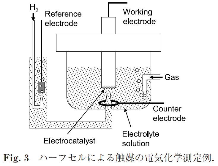
Fig. 4(a)にグラッシーカーボン電極に固定した白金担持カーボン(Pt/C 触媒)の酸素還元反応の対流ボルタモグラムを示す.電極電位を下げていくと,E< 1 V で酸素還元電流i が流れ始め,電極回転数に応じた拡散限界電流iLに達した後は一定となる.拡散限界電流に達するまでの電流は,対流による拡散と反応活性化の混合支配となっており,次のような関係で表される.
1/i = 1/ik+ 1/iL (2)
ここで,ik は拡散の影響を除いた活性支配電流である.式(2)を変形するとikは次のように表される.
ik= i・iL/(iL- i) (3)
このようにi とiLより得られる活性支配電流ikを用い,電極活性の評価指標として用いられる比活性is(specific acticity),質量活性im(mass activity)は次のように求められる.
is (mA/cm2Pt)= ik (mA)/Ptの活性表面積(cm2Pt) (4)
im(mA/mgPt)= ik (mA)/Pt担持量(mgPt) (5)
ここで,触媒の活性表面積(Electrochemically activesurface area; ECSA)は後述のCV を用いて決定することができる.
Fig. 4(a)の対流ボルタモグラムより,式(3),(4)を用いて得られるisの電位依存性(ターフェルプロット)をFig.4(b)に示す.式(3)用いた手法は簡便であるが,iLとi の差をとるため,i がiLに近づくと実験誤差やノイズの影響が大きくなる.また,電極活性が低く拡散支配領域が観察できない(iLを決定できない)場合は適用不能となるため,電極回転速度の異なる対流ボルタモグラムをいくつか測定し,Koutecky-Levich プロット(式(6))を用いた解析が必要になる.
1/i = 1/ik+ 1/(0.62nFACD2/3ν−1/6ω1/2) (6)
ここで,nは反応電子数,Fはファラデー定数(96485 C mol−1),Aは電極の幾何面積(cm2),Cは反応化学種濃度(mol cm−3),D は反応化学種の拡散係数 cm2s−1),ν は溶液の動粘度( cm2 s−1), ω は電極の回転角速度( rad s−1) である.Koutecky-Levich プロットは,1/i をω−1/2に対してプロットして得られる直線をω−1/2= 0 に外挿して1/ikを求めるのでiLが明確でない場合でも解析が可能となる.解析の詳細は成書などを参照していただきたい1,5,6).

3 サイクリックボルタンメトリー(CV)
PEFC におけるCV の主要な用途のひとつに活性表面積(ECSA)測定が挙げられる.触媒の活性表面積の大小は電極活性を左右する要因であるので,初期活性・劣化解析のど
の場合においても重要な指標となる.また,PEFC の電極では通常,仕込んだすべての触媒が利用できるわけではなく,同じ触媒材料を使っても触媒層の形成法や作動条件によって触媒電極の中での実際に使える白金の割合(すなわち白金利用率)は変わってくる.CV はハーフセルだけでなく,MEAを用いた測定でも,触媒の活性表面積を簡便に“その場”測定できる解析法である.白金触媒電極の活性表面積評価では,水素吸脱着波の電気量による方法が用いられることが多い.これは,表面積測定のために特別なガスや装置が不要であること,白金表面の水素吸着がアンダーポテンシャル析出(UPD)の機構で進行しマルチレイヤー析出などが起こりにくいこと,清浄な電極では明確なピークが得られることなどによる.
3. 1 ハーフセルを用いたCV 測定
測定は分極測定の場合と同様,触媒をグラッシーカーボン電極に固定化して行う.Fig. 5 に0.1 M 過塩素酸水溶液中での白金電極の典型的なCV の例を示す(電流の符号は酸化電
流をプラスとして表示).

0.4 V よりも卑な電位領域で水素の吸脱着ピークが現れる.水素吸着の電気量QHは,Fig. 5 の斜線で示した電気二重層容量電流(水平線)と水素発生ピーク立ち上がり点(垂直線)で囲まれた領域とする.
3. 2 MEA(単セル)を用いたCV 測定
単セルでの発電に寄与可能な活性表面積を求めるにはMEA を用いて単セルを組み,CV 測定を行う.測定上の注意点は,ハーフセルの場合と同様である.セルを室温付近
(あるいは発電時の温度)に保温し,試験極・対極に加湿窒素ガスを流す.試験セル両極内の空気が完全に置換した後,対極側に加湿水素ガスを流し水素雰囲気とする.
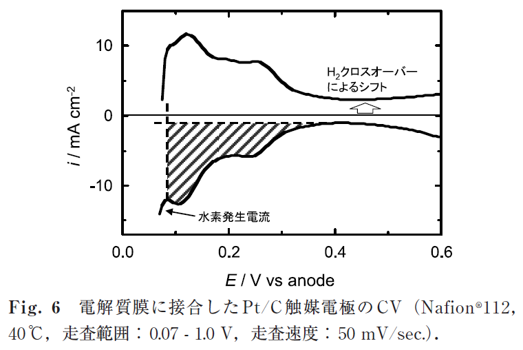
ガス拡散電極を用いるMEA でのCV 測定では,水素発生および発生した水素ガスの酸化電流がハーフセルの場合よりもかなり高い電位(~ 0.1 V)から流れ始めることが多く,水素吸脱着波の電流に重なって現れるため,QH計算の誤差原因になりやすい.このような水素発生の電位シフトは,作用極触媒近傍の水素分圧が低下するために生じると報告されており10),これを防ぐためにはCV 測定時に試験極パージ窒素ガスの流量を絞る,もしくは止めることが有効とされている7,10).
Fig. 6 にPt/C 触媒電極のCV を示す.パターン全体が酸化電流側にシフトする点を除けば,基本的に電解質水溶液中で測定した場合と同様のCV が得られる.このCV シフトは,水素ガスクロスオーバーの影響である.特に薄いフッ素系電解質膜の系ではクロスオーバー水素量が多く(~ 1 mA/cm2の電流に相当),CV の電流値に重畳するクロスオーバー水素の酸化電流も大きくなる.このようにMEA で求めた電極の有効活性表面積(SAMEA)とハーフセル測定などで求めた触媒材料固有の活性表面積(SAcat)との比より白金利用率uPtを決定できる.
uPt=SAMEA/SAcat (8)
uPtを求める手法としては,後述する一酸化炭素(CO)ストリッピング/CO吸着を利用する手法も提案されている11).
3. 3 CV の応用例1 - 触媒加速劣化・解析-
PEFC の耐久性向上は実用化に向けた重要な課題の1 つであり12),劣化要因の1 つである触媒劣化を抑制することが求められている.通常のPEFC の運転条件では,触媒の劣化現象はゆっくりと進行することが多く,材料やシステムの開発を促進するためには,適切な劣化加速手法とその評価法の確立が重要である.このような目的で,ハーフセルおよびMEA に対して,CV などの電位サイクルを用いる触媒劣化加速評価法が,燃料電池実用化推進協議会(FCCJ)から提案されている(ただし,その後の新たな知見を基に評価法は今後改訂される可能性がある)13).
Pt/C 触媒(特にカソード)劣化の主要因は,Pt 微粒子の溶解・凝集および触媒担体劣化と考えられている.Pt 溶解はPt の酸・還元を繰り返すことで加速されることが知られているが14),このような環境はOCV と負荷状態を繰り返す負荷変動時のカソード側の条件によくあてはまる.Fig. 7(a)にFCCJ より提案されているMEA での負荷変動試験条件を示す.窒素雰囲気下0.6 V/0.9 V の間で電位サイクルを行うことでPt の酸化還元を繰り返し,Pt 溶解が加速される条件下での触媒安定性を評価する試験法である.
一方,カーボンブラックなどの触媒担体の劣化は1 V を超える高電位で加速されることが知られている15).通常の状態であれば,燃料電池電極がこのような高い電位にさらされることはないが,例えば起動停止時には逆電流機構とよばれるメカニズムでカソード電位が最大1.5 Vに達することがある16).このような状態を模擬する起動停止試験としてFig. 7(b)に示すような試験条件が提案されている.窒素雰囲気下0.9V/1.3 V の矩形波サイクルを繰り返すことで,起動停止時の異常電位に対する耐性を評価する.

MEA のPt/C カソード触媒電極にFig. 7(b)の起動停止試験を2000サイクル実施した例をFig. 8 に示す.サイクルを重ねるにつれて水素吸脱着波や酸化物層生成・還元ピークが縮小しており,Pt の溶解・凝集が進行していると考えられる.同時に電気二重層電流も徐々に増加し,0.5 - 0.6 V 付近にはカーボン表面の官能基によるレドックスと考えられるピーク対が次第に明確になっていることから,カーボン担体表面の酸化が進行していることも示唆される.CV の水素吸脱着波からECSA を求め,初期値で規格化した値をサイクル数に対してプロットした結果をFig. 8(b)に示す.なお,Fig.8 の例は80 ℃でのCV 測定であるため,水素被覆率低下や水素発生の影響が無視できず正確なECSA 評価は困難になる.しかし,Fig. 8(b)のようなサイクルに伴う相対的な変化を議論することは可能である.ハーフセルを用いる加速劣化試験法については,負荷変動・起動停止試験ともに三角波CV の繰り返しが提案されている13).Fig. 9 にPt/C 触媒のハーフセルによる起動停止試験(CV三角波1.0 V/1.4 V)を10000サイクル実施した例を示す.Fig. 8 のMEA の結果と同様にECSA の減少と共に二重層容量の増大が確認できる.


8月13日(金)
MD シミュレーションを用いたアイオノマー薄膜の構造およびプロトン輸送の解析
小林 光一他著、燃料電池 Vol.18 No.4 2019
概要:固体高分子形燃料電池(PEFC:Polymer Electrolyte Fuel Cell)は車載用電源や定置用電源として盛んに研究・開発が行われてきた。発電時、PEFC 内部ではプロトンや水素、酸素といった様々な物質が輸送されるため、PEFCの性能向上のためには内部の輸送現象を理解する必要がある。本研究では触媒層内アイオノマー薄膜においてアイオ
ノマー膜厚が膜構造とプロトンの輸送特性にもたらす影響について解析を行った。本研究では分子動力学シミュレーションを用いてナノスケールの構造と輸送について評価を行った。本研究の結果より、アイオノマー膜厚が膜内部の水分子の分布に影響を与え、アイオノマー膜厚がおよそ7nm において最も水クラスターの接続性が高く、プロトン
の自己拡散係数も高くなることが分かった。
1.緒言
固 体 高 分 子 形 燃 料 電 池(Polymer Electrolyte FuelCell:PEFC)は今後我が国が水素社会へと舵を切っていく上で、特に車載用や家庭用電源といったシーンにおいてその性能が期待され、盛んに開発が行われている。PEFCを広く普及させるためには単位セルの出力密度向上が欠かせない1)。このためには膜電極接合体(Membrane Electrode Assembly:MEA)において分子レベルで構造と輸送の相関を明らかにする必要があり、特に触媒層においてはガスの拡散性、プロトン・電子の伝導性を考慮した構造
の最適化が求められる2)。
・・・・・・・・・・・・・・・・・・・・
2.計算手法
本研究では炭素壁面上にアイオノマー薄膜が吸着した計算系を作成し、アイオノマー薄膜の膜厚が膜の構造およびプロトン輸送特性に与える影響について分子動力学シミュ
レーションを用いて解析を行った。以下に計算系の構成を述べる。アイオノマー薄膜には Nafion® のモデルを用いた。用 い た Nafion® の 等 価 質 量(Equivalent Weight:EW)は 1146 であり分子構造は図1に示す通りである。また、解析の精度を保ったまま計算負荷を低減するため、CFnの原子群を1原子として扱う United Atom(UA)モデル 14)を用いた。アイオノマー薄膜の膜厚は系内の Nafion®の本数を変化させることで制御した。アイオノマー薄膜の膜厚は膜の含水率などによって±1nm ほど変化するが、系内の Nafion® 本数とアイオノマー膜厚の目安を表1にまとめた。
・・・・・・・・・・・・・・・・・・・・
3.結果と考察
3.1 最大クラスター長
まずアイオノマー薄膜の膜厚と膜内の水クラスター構造の相関を解析するために、クラスターサイズの解析を行った。本計算では水・ヒドロニウムイオンの酸素原子の再隣
接原子間距離が 3.3Å 以内にある集合体を水クラスターと定義した。この 3.3Å という距離は Nafion® バルク膜における水分子の酸素原子間の RDF における第一ピークの終端値である 20)。本研究ではクラスターに含まれる水分子数をクラスターサイズとして定義している。図4にλ =3、14 において膜厚を変化させた時の平均クラスターサイズを示した。λ =14 においてはクラスターサイズが膜厚と共に増加する一方、λ =3においてはクラスターサイズに大きな変化がないことがわかる。一般に膜内のクラスターが成長することで、プロトンの自己拡散係数は増加するが、薄膜の場合はクラスターが壁面垂直方向に成長しても水平方向の自己拡散係数への影響が少ないことが考えられる。
・・・・・・・・・・・・・・・・・・・・
3.2 密度分布
本研究で扱っている炭素壁面上のアイオノマー薄膜の系では、炭素壁面や界面の影響により壁面垂直方向の密度は非一様になっていると考えられる。このような系の密度分
布を求めるため、系内を x×y×z = 1.02 × 0.88 × 1.00Å3の微小なセルに分割してセルごとの密度ρlocal を求めた。またρlocal を壁面水平方向について平均化することによって壁面垂直方向の密度分布を求めた。
・・・・・・・・・・・・・・・・・・・・
3.3 プロトン自己拡散係数
最後にプロトンの輸送特性とアイオノマー薄膜の膜厚の関係を解析するために、プロトンの自己拡散係数を計算した。拡散係数は平均二乗変位(Mean Square Displacement:MSD)から Einstein の式を用いて計算した。MSDの計算式は式 (2)、(3) に示し、Einstein の式を式 (4) に示した。なお、自己拡散係数は図2に示すように炭素壁面に対して水平方向に限定した。これは、電解質膜から触媒までのプロトン輸送を考えたとき、炭素壁面に対して水平方向の輸送が大部分を占めるためである。
・・・・・・・・・・・・・・・・・・・・
4.結言
本研究では MD シミュレーションを用いて PEFC アイオノマー薄膜におけるプロトン輸送特性について解析を行った。プロトンの拡散モデルにaTS-EVB モデルを用いてグロッタス機構による拡散を考慮したプロトン輸送特性の解析を実施した。またアイオノマー薄膜のモデルとして、接触角 90°の炭素壁面を模擬した LJ 壁上に Nafion® 粗視化モデルを吸着させて、アイオノマー薄膜の膜厚を変化させることでプロトン輸送特性や膜構造の変化を解析した。 まずλ= 14 (RH=100%におけるバルクNafion膜中の含水率に相当する)においてはプロトンの自己拡散係数とクラスター接続性に膜厚依存性が少ないことがわかった。また、クラスター長は計算領域の大きさとほぼ等しく、これは高含水率時にクラスターが完全に接続していることを示唆している。さらに膜厚増加とともにクラスターは壁面垂直方向に成長しており、これがλ= 14 の時にプロトン自己拡散係数の膜厚依存性が小さいことの一因であると考えられる。
・・・・・・・・・・・・・・・・・・・・
面白そうな論文がある。ちょっと覗いてみよう。なんか、これは、凄い結果が得られているようだ!
High Pressure Nitrogen-Infused Ultrastable Fuel Cell Catalyst for Oxygen Reduction Reaction, Eunjik Lee et al., ACS Catal., 11, 5525−5531 (2021)
ABSTRACT:
The mass activity of a Pt-based catalyst can be sustained throughout the fuel cell vehicle life by optimizing its stability under the conditions of an oxygen reduction reaction (ORR) that drives the cells. Here, we demonstrate improvement in the stability of a readily available PtCo core−shell nanoparticle catalyst over 1 million cycles by maintaining its electrochemical surface area by regulating the amount of nitrogen doped into the nanoparticles. The high pressure nitrogen-infused PtCo/C catalyst exhibited a 2-fold increase in mass activity and a 5-fold increase in durability compared with commercial Pt/C, exhibiting a retention of 80% of the initial mass activity after 180 000 cycles and maintaining the core−shell structure even after 1 000 000 cycles of accelerated stress tests. Synchrotron studies coupled with pair distribution function analysis reveal that inducing a higher amount of nitrogen in core−shell nanoparticles increases the catalyst durability.
Ptベースの触媒の質量活性は、セルを駆動する酸素還元反応(ORR)の条件下でその安定性を最適化することにより、燃料電池車の寿命全体にわたって維持できます。 ここでは、ナノ粒子にドープされた窒素の量を調整することによってその電気化学的表面積を維持することにより、100万サイクルにわたって容易に入手可能なPtCoコアシェルナノ粒子触媒の安定性の改善を示します。 高圧窒素注入PtCo / C触媒は、市販のPt / Cと比較して質量活性が2倍に増加し、耐久性が5倍に増加し、18万サイクル後に初期質量活性の80%の保持を示しました。 1 000000サイクルの加速応力試験後もコアシェル構造を維持します。 ペア分布関数分析と組み合わせたシンクロトロン研究は、コアシェルナノ粒子に大量の窒素をドープすると触媒の耐久性が向上することを明らかにしています。

INTRODUCTION
Extensive practical applications of the commercial hydrogen fuel cell vehicle have been delayed because of the high cost and limited durability of the membrane electrode assembly (MEA).
One of the main reasons for the high cost of the MEA is the large amount of Pt used to catalyze the oxygen reduction reaction (ORR) at the cathode of the proton exchange membrane (PEM) fuel cell.
In the past decade, several studies investigated ORR electrocatalysts to reduce the cost of the MEA.
One of the main strategies is to add modifiers to the Pt catalyst by changing the structure and morphology of the PtM (metal) alloy catalyst, while others include completely avoiding Pt usage by using various nonprecious M−N−C moiety catalysts.
Although the addition of modifiers can drastically increase catalytic performance, it cannot be sustained for prolonged periods, which is a major factor impeding commercialization.
To date, carbon-supported PtCo alloy nanoparticles have emerged as the best alternative to Pt/C; original equipment manufacturers are already using them in first-generation
hydrogen fuel cell vehicles.
For better Pt utilization efficiency throughout the fuel cell lifetime, an ideal catalyst should be able to maintain its electrochemical surface area (ECSA).
Although earlier studies have corroborated nitrogen’s role in stabilizing the catalyst, high pressures doping of nitrogen in a controlled environment on industrial scale core−shell nanoparticles was not achieved.
先に試して失敗したものを、今回成功させた、ということで、その先導研究を見たら、同じ研究グループのようで、安心した。それが以下の2件。
(25) Kuttiyiel, K. A.; Sasaki, K.; Choi, Y.; Su, D.; Liu, P.; Adzic, R. R. Nitride Stabilized PtNi Core−Shell Nanocatalyst for high Oxygen Reduction Activity. Nano Lett. 2012, 12 (12), 6266−6271.
(26) Kuttiyiel, K. A.; Choi, Y.; Hwang, S.-M.; Park, G.-G.; Yang, T.- H.; Su, D.; Sasaki, K.; Liu, P.; Adzic, R. R. Enhancement of the oxygen reduction on nitride stabilized Pt-M (M = Fe, Co, and Ni) core−shell nanoparticle electrocatalysts. Nano Energy 2015, 13, 442−449.
Thus, in this study, to obtain a highly stable and active ORR catalyst, a highpressure nitriding reactor that can infuse a controlled number of nitrogen (N) atoms into the alloy nanoparticles was developed.
Varying the ratio of N atoms in the PtCo/C core−shell nanoparticles can significantly affect the morphology of the nanoparticles and simultaneously increase their stability
without impacting the activity.
Herein, we report the preparation of N-stabilized PtCo core−shell nanoparticles with ultrastable configurations; the result is a highly durable ORR catalyst that can withstand up to 1 000 000 cycles in accelerated stress tests (ASTs), enabling rapid commercialization of fuel cell vehicles.
To the best of our knowledge, thus far, no catalysts have been reported that can last 1 million cycles.
The best configuration (Pt40Co36N24/C) retained 93% of its ECSA, while its initial half-wave potential decreased by only 6 mV after 30 000 cycles.
This confirms that the proposed configuration is a suitable alternative to the commercial Pt/C catalyst, whose ECSA deteriorated by 40% under similar conditions.
CONCLUSION
We exhibited that nanostructured core−shell materials with high contents of N in their cores can be engineered to sustain harsh and oxidative electrochemical environments during fuel cell operation.
X-ray experiments and PDF analyses revealed that a high N content could protect the Co core against dissolution.
The sustainment of 1 million cycles after harsh and corrosive ASTs without significant dissolution facilitates the potential industrial scale application of the catalysts.
This strategy presents a promising approach to develop cheap and ultradurable core−shell catalysts using other 3d transition metal cores.
8月14日(土)
High Pressure Nitrogen-Infused Ultrastable Fuel Cell Catalyst for Oxygen Reduction Reaction, Eunjik Lee et al., ACS Catal., 11, 5525−5531 (2021)
RESULTS AND DISCUSSION
Carbon-supported PtCo core−shell nanoparticles were prepared by reducing platinum acetylacetonate [Pt(acac)2] and cobalt acetylacetonate [Co(acac)2] via ultrasound-assisted polyol synthesis.
Transmission electron microscopy (TEM) analysis showed that the as-synthesized PtCo nanoparticles exhibited a core−shell structure with an average particle size of ∼2.3 nm (Figure S1).

Scanning TEM (STEM) and energy dispersive X-ray spectroscopy (EDS) confirmed the core−shell structure with 1−2 Pt monolayers on the Co-rich core (Figure 1B−D).

The PtCo core−shell nanoparticles were annealed in an argon/ammonia mixture (N2/NH33: 5/95) at 510 °C in three pressurized environments (1, 40, and 80 bar).
The nanoparticles maintained their core−shell structures and exhibited an increase in the particle size and a change in composition (Figure 1F−H).

As shown in Figure 1E, higher pressure increases the N content in the nanoparticles but ultimately decreases the particle size.

On the basis of the N content in the nanoparticles, the molar ratio changes drastically; the resultant nanoparticles are denoted as Pt52Co48/C, Pt53Co45N2/C, Pt44Co42N14/C, and Pt40Co36N24/C (Table 1).

For all samples, in-house X-ray diffraction (XRD) patterns exhibit the typical face-centeredcubic (fcc) structure, with no phase segregation, corresponding to Pt and its alloys with transition metals (JCPDS, No. 87- 0646) (Figure 1A).

The position of the (111) peak of PtCo/C shifts to a higher angle compared with that of Pt/C, indicating that Co atoms with relatively smaller atomic sizes are incorporated into the Pt lattice, causing compressive strain.
Interestingly, the nitriding pressure directly affects the full width at half-maximum (fwhm) and position of the (111) peak.
In particular, the fwhm increases and the (111) peak position gradually shifts to a lower angle with an increase in the nitriding pressure.
This suggests that the nitriding pressure changes the atomic structure of the catalyst particles while relaxing the lattice mismatch between Pt skin and cobalt nitride core (Table 1).
Furthermore, X-ray photoelectron spectroscopy (XPS) studies indicate that, compared with metallic Pt, the Pt 4f peak in all samples shifts to a lower binding energy (BE), likely owing to the charge transfer from Co to Pt (Figure S2).

Additionally, no peaks (∼399.8 eV) for imides/lactams/amides are observed, indicating that most N in the samples exists in the form of nitrides.
To gain further insights about how the as-synthesized PtCo core−shell nanoparticles maintain their structures while incorporating N atoms, we carried out ab initio molecular
dynamics (AIMD) studies to simulate the formation of the CoN nanophase in the nanoparticle core.
Before the conduction of AIMD, the NH3 molecules were packed into a unit cell with cuboctahedral PtCo nanoparticles under pressures of 1, 10, and 45 bar by use of the COMPASSII force field.
We considered the entropic effect to identify the continuous reaction process incorporated at a finite temperature of 783 K.
In the case of a single PtCo nanoparticle, it is found that N atoms from the NH3 molecules cannot penetrate the Co core even at a high pressure of NH3, as shown in Figure S3 and Movie S1.
Therefore, we tested the case of formation of PtCoN core−shell nanoparticles through a particle growth process involving the agglomeration of the preformed PtCo fragments into nitride cores that are consequently covered by a Pt shell.
The results shown in Figure 2A indicate that this is the likely mechanism of the particle size increasing from ∼2.3 nm for pure PtCo nanoparticles to ∼4.2 nm for Pt53Co45N2/C (Table 1).

Interestingly, AIMD studies are appreciably consistent with the observation that two Pt12Co1 nanoparticles at 10 bar of NH3 (e.g., 28.7 bar at 783 K) can spontaneously merge without any considerable activation barrier.
The simulations indicate the formation of irregular particles with a compressed Pt−Pt distance depending on the location of nearby N atoms, as revealed by the atomic pair distribution function (PDF) analysis and the reverse Monte Carlo modeling (discussed below), thereby increasing the number of N atoms that exist near the Pt sublayer.
In situ Co K edge X-ray absorption near-edge structure (XANES) spectra of Pt52Co48/C, Pt53Co45N2/C, Pt44Co42N14/ C, and Pt40Co36N24/C nanoparticles (Figure 2B) were
obtained in 0.1 M HClO4 at a potential of 0.42 V.

As the N concentration increases, the peak intensity at 7724 eV starts decreasing; the highest peak at 7727 eV is observed at a N concentration of >14 at%.
This change can be ascribed to a change in the electronic structures of Co due to N doping.
As shown in Figure S7, the XANES spectra of CoO (Co2+) and Co3O4 (Co2.67+) exhibit the highest peaks at 7725 and 7729 eV, respectively; meanwhile, the highest peak for Pt40Co36N24/C lies between them.

Thus, the N doping of PtCo catalysts alters the electronic state of Co, resulting in an increase in the oxidation state.
The increase in the oxidation state with an increase in the N content is also supported by the data shown in the inset of Figure 2B; half-step energy values (at 0.5 of the normalized absorption in the XANES spectra) increase with an increase in the N concentration.
Figure 2C shows the in situ Pt L3 edge XANES spectra of the PtCo/C and N−PtCo/C catalysts measured in 0.1 M HClO4 at a potential of 0.42 V.

The intensities of the white lines (first peaks in XANES data) change with the variation in the N content in the N−PtCo/C catalysts.
As shown in the inset of Figure 2C, the intensity increases with increase in N concentration; it is higher than that of a Pt foil but lower than that of the PtCo/C catalyst.
The change in white line intensity is related to the d-band structure in Pt. It is well-known that higher intensities correspond to an increase in d-band vacancy; that in turn lowers the adsorption of the intermediate molecules (such as OOH and OH) on the Pt surface.
Thus, N doping can weaken the interaction of the Pt surface with oxygen, compared with that of bulk Pt.
However, the effect is not as strong as that for the PtCo/C catalyst as the white line intensity for the N−PtCo/C catalysts is lower than that of PtCo/C and varies with the N content.
The XANES data suggest that N doping in N−PtCo/ C alters the electronic states of Co and Pt, resulting in moderate adsorption strength of oxygen on the Pt surface.
To comprehensively understand the particle structure, highenergy synchrotron XRD experiments coupled with atomic PDF analysis were carried out.
Experimental PDFs (Figure S8) were fit with 3D models for the nanoparticles using classical molecular dynamics (MD) simulations and were further refined against the experimental PDF data by employing reverse Monte Carlo modeling.
Cross sections of the models emphasizing the core−shell characteristics of the particles are shown in Figure 3.
The models exhibit a distorted fcc-type structure and reproduce the experimental data in exceedingly good detail (Figure S8).
The bonding distances between the surface Pt atoms and surface Pt coordination numbers extracted from the models are also shown in Figure 3.
As observed, PtCo core−shell particles exhibit large structural distortions (∼1.8%).
The surface Pt−Pt distance in Pt53Co45N2 is 2.739 Å, which is approximately 1.5% shorter than the surface Pt−Pt distances in bulk Pt (2.765 Å).
Furthermore, the surface Pt−Pt distance in PtCo is 2.731 Å, indicating 0.3% more strain compared with the strain observed in the Pt53Co45N2 particles.
This indicates that N relaxes the compressive stress in PtCo core−shell particles.
Moreover, the average surface Pt coordination number for the particles with CoN cores increases and becomes more evenly distributed than in the case of pure Pt particles; that is, the surfaces of N-treated particles appear less rough (fewer undercoordinated sharp edges and corners), which can affect the binding strength of oxygen molecules to the particle surface and accelerate the ORR kinetics.
As expected, the N-treated particles show an increased number of N atoms located near the Pt shell, which explains the increased stability of the nanoparticles compared with those of pure Pt and PtCo particles.
The electrochemical performances of all the catalysts were compared using cyclic voltammetry (CV) curves (Figure S4).
The incorporation of Co into the Pt nanoparticles increases the ECSAs of the catalysts, while that of N into the PtCo nanoparticles decreases their ECSAs (Figure 4A).

A slightly different trend was observed with respect to the specific and mass activities of the catalyst (Figure 4B).

The PtCo/C catalyst with low nitrogen content shows the highest activity among the catalysts; however, an increase in N content does not drastically change its catalytic behavior.
Our study was mainly focused on achieving structural stability of the catalyst.
AST cycles at 0.6−0.95 V and 3 s hold were employed for each catalyst.
All N-infused PtCo/C catalysts showed higher stability and activity compared with commercially available Pt/C and PtCo/C catalysts (Figure S5).

The catalyst with the highest N amount (Pt40Co36N24/C) retained 93% of its ECSA, with a decrease of only 6 mV in its initial half-wave potential after 30 000 cycles.
To further investigate the structural integrity of all the catalysts, we cycled them until the ORR activity decreased to half its initial value.
As observed in Figure 4C, most of the N-infused catalysts retained their structures up to 230 000 cycles; however, the catalyst with the highest amount of N (Pt40Co36N24/C) retained its structural integrity until 1 000 000 cycles and lost just 44 mV from its initial half-wave potential (Figure S6).


Fuel cell (25 cm2) performance tests with 0.1 mg cm−2 Pt content showed promising results (Figure 4D,E). The Pt40Co36N24/C catalyst achieves the U.S.
Department of Energy durability target of a 30 mV voltage drop at 0.8 A cm−2 after 30 000 ASTs (Figure 4H).
Moreover, considering the particle size growth after 30 000 ASTs, the PtCo nanoparticles grew by 41% from their initial average size (Figure 4F), whereas the N-infused PtCo nanoparticles grew by 21%, confirming that N plays a key role in impeding nanoparticle coarsening (Figure 4G).
As previously reported, DFT-based studies clearly support the higher ORR activities of
nitride-stabilized Pt−metal electrocatalysts over Pt/C catalysts.
Their volcano-like trends show that the interactions of Pt/C and PtCo/C with oxygen are significantly stronger and weaker, respectively, compared with those of PtCoN/C.
The outstanding stability of high-pressure N-infused PtCoN/C catalysts can be easily explained on the basis of our resent DFT findings.
The segregation effect of Pt facilitated by the higher N concentration in turn facilitates the diffusion of Pt atoms to the vacant sites of the outermost shell, preventing dissolution.
Evidently, these results demonstrate the enhanced catalytic stability of the Pt40Co36N24/C catalyst over the other N-infused PtCo catalyst.
次のレビューは、様々な触媒の作り方が、網羅的に紹介されている。
Ultra‑low loading of platinum in proton exchange membrane‑based fuel cells: a brief review, Aristatil Ganesan and Mani Narayanasamy, Materials for Renewable and Sustainable Energy (2019) 8:18
Abstract
This review report summarizes diferent synthesis methods of PEM-based fuel cell catalysts with a focus on ultra-low loading of Pt catalysts. It also demonstrates fuel cell performances with ultra-low loading of Pt catalysts which have been reported so far, and suggests a combination method of synthesis for an efficient fuel cell performance at a low loading of Pt catalyst. Here, maximum mass-specifc power density (MSPD) values are calculated from various reported performance values and are discussed, and compared with the Department of Energy (DOE) 2020 target values.
Introduction
・・・・・・・・・・
Regrettably, expensive platinum group metal (PGM) catalysts block the commercial sales/volume. PGMs (plus application) cost contribute to the total cost of FC stack
from 21% (1000 FC systems/year) to 45% (500,000 systems/year) [5] as expected. Since PGMs are expensive, the PGMs loading should be reduced from current (target) levels. As
PGMs play a critical role in both hydrogen oxidation reaction (anode–HOR) and oxygen reduction reaction (cathode– ORR) of the fuel cell, the challenge is ahead in the PEMFC community to address PGM cost issues for its use in both anode and cathode of the fuel cell.
・・・・・・・・・・
According to DOE 2020, the loading target of PGM is 0.125 mgcm−2 and < 0.1 mgcm−2 for the anode and cathode, respectively. Nevertheless, a still lower loading of about 0.0625 mgcm−2 is required for PEMFC vehicles to stand along with IC engine vehicles.
Literature
Many research groups are working on Pt alloy catalysts such as PtCo; PtNi; PtCoMn; WSnMo; PtRu; PtAgRu; PtAuRu; PtRhRu; and Pt–Ru–W2C to replace Pt/C [7–10]. By providing high surface area carbon supports, Pt content could be reduced with high Pt utilization [11, 12]. Using the plasma sputtering technique [13], the total Pt loading in both anode and cathode is reduced to 20 μgcm−2. By this method, uniform dispersion of Pt as clusters with size less than 2 nm is achieved with high catalyst utilization.
Most researchers have made an attempt to reduce Pt loading by providing novel catalyst supports such as multiwalled CNT and single-walled CNT [14]. Binary alloys of Pt, Pt–Cu [15], Pt–Co [16–19], Pt–Ni [17, 18], Pt–Cr [17] revealed 2–3 times higher mass-specific activity than Pt/C, which is due to alloy effects and ligand effects. A ternary alloy of PtFeNi and PtFeCo [19] showed excellent ORR activity, but in some cases presents Pt particles aggregation. A bimetallic alloy of Pd–Pt on hollow core mesoporous shell carbon (PtPd/HCMSC) demonstrated enhanced ORR activity and stability [20, 21]. Recently, a core shell of PtCo@Pt offered low loading of catalyst, but it had a disadvantage of base metal cobalt (Co) leaching (dissolution) from bulk to surface [22]. Wang et al. [21] investigated PtNi alloy as a high-performing catalyst for automotive applications with a low loading of Pt: 0.125 mgcm−2 which satisfied the DOE 2020 target.
Pt–Ni alloy catalyst synthesized by direct current magnetron sputtering involves Pt sputtering on synthesized PtNi/C substrate which forms multilayered Pt-skin surface,
with superior ORR activity. This catalyst involves the mature technology of synthesis with improved performance compared to Pt/C. Though this catalyst presents superior performance, it involves careful preparation of Pt target material for sputtering (costly), preparation of PtNi by chemical reduction, thermal decomposition, and acid treatment with final heat treatment. Materials’ preparation involves many steps and needs careful optimization for getting a reasonable yield of catalyst. Durability studies were not conducted at the MEA level as it is specified by DOE.
Kongkanand et al. investigated [22] PtCo on high surface area carbon (HSC), which demonstrates a less degree of PtCo particle coalescence after the stability test. Also,
HSC is favored for start-up performance and long-term durability. The dissolution of Pt and Co was resolved by developing a deposition model [23]. DOE has updated its
cost estimation for an automotive fuel cell by 15%, i.e., $45/ kW, because of the development of catalyst, PtCo/HSC. This catalyst system would reduce the total cost of the system to 14% or $7.5/kW [22]. These catalysts (PtNi/PtCo) cost about $15.20/g for cathode (Pt 0.100 mgcm−2) and $10.86/g for Anode (Pt 0.025 mgcm−2) [1]. Chen et al. investigated Pt3Ni nanoframes and demonstrated high mass activity with durability, but MEA performance at high current density was challenging [23]. The shape-controlled synthesis of Pt–Pd and Ru–Rh catalyst showed high mass activity and it offers a commercially efficient scale-up method. This catalyst has issues with performance at the MEA level and stability [24]. In addition to catalyst support modification, and alloying of
Pt, for Pt content reduction, a proper MEA fabrication methodology is to be identified for low Pt loading. This review provides intensive guidance for researchers working on low
Pt loading catalyst for fuel cells.
Most promising methods for the preparation of electrodes
Though there are several methods such as physical vapor deposition, chemical vapor deposition, sputter deposition, galvanic replacement reaction (Pd nanocrystals with different shapes) [24] hydrothermal synthesis [25] electrodeposition (hetero-structured nanotube dual catalyst) [26] electrospinning [27] and molten salt method [28], electrodeposition [29] are available for catalyst synthesis and coating, only very few methods are practically feasible for producing nanoparticles of a catalyst and its efficacy for coating on electrodes.
Electrodeposition
The need and necessity for nanostructured energy materials with high surface area, and for its efficient application in energy conversion devices, can be achieved only with the
electrochemical synthesis route. Electrodeposition technique proves to be the best method for the following reasons.
1. Electrode potential, deposition potentials, current densities, and bath concentrations could be controlled for the synthesis of homogenous nanostructured materials.
Hence by varying deposition parameters, one can synthesize thin catalyst film, with desired stoichiometry, thickness, and microstructure.
2. Particle size, desired surface morphology, catalyst loading, thickness, and microstructure can be easily achieved using various control parameters involved in
electroplating.
3. Electrochemical reactions proceeded at ambient temperature and pressure, as high thermodynamic efficiency during plating is maintained.
4. Environmentally friendly.
5. Synthesis can be started with low-cost chemicals as precursor materials.
6. One-pot single-step synthesis of the final product is possible by avoiding a number of steps.
7. Any metal or alloy can be easily doped into desired nanostructured materials.
8. The required nanostructured energy materials can be directly grown on the electrode surface by electrochemical method, and it provides good adhesion, large surface area, and electrical conductivity.
And hence, this method is found suitable for construction of energy devices with high efficiency and with low cost.
9. By this method, materials with poor electrical conductivity of metal oxide used as catalyst supports can be easily incorporated into advanced energy materials and will facilitate fast electron transport mechanism. Therefore, electrical conductivity of catalyst supports can be enhanced by the electrodeposition method.
10. The electrochemical synthesis route eliminates the complexity of mixing catalyst powders with carbon black and polymer binder in fabricating electrodes for fuel cells in a short time [29].
・・・・・・・・・・
Chemical precipitation method
A thin nanocatalyst layer is formed by the reduction of reducing agent in the precursor solution. The desired particle size of the catalyst can be achieved by varying parameters,
such as temperature, pH, the ratio of reducing ion to Pt, reaction time, and stirring rate. The main disadvantage of this method is producing irregular particle size and shape, and resulting in the inhomogeneous layer. This formation is due to various growth kinetics and conditions, and thus it is least used for catalyst synthesis.
Colloidal method
By this method, colloidal dispersion is formed by stabilizer and the precursor. The suitable support material is added and by which colloid deposition occurs on the support surface. In the final stage, the decomposition of colloid results in the formation of catalyst. The common colloidal particles formed by the precursors, H2PtCl6 and RuCl3,
and reduced with reducing agent. The stabilizers and reducing agents present in the final product will have to be removed by thermal treatment. This method involves various steps to be followed for the catalyst synthesis.
Sol–gel synthesis method
This method allows forming solid particles suspended in liquid solution (sol) and upon subsequent aging, and drying to form a semi-solid suspension in a liquid (gel). And subsequent calcination results in a mesoporous solid or powder formed on the substrate. Pore size distribution on the catalyst layer can be varied by various experimental parameters. The disadvantage associated with this technique is catalytic burning in pores, makes them inaccessible to reactants, and resulting in low catalyst utilization.
Impregnation method
This method uses high surface area carbon supports for the formation of catalyst. In this method, chloride Pt salt directly mixed with reducing agents, Na2S2O3, NaBH4, N2H4,
formic acid, and H2 gas in an aqueous solvent. This method results in Pt agglomeration and weak support due to the high surface tension of the liquid solution [56].
Microemulsion method
The water-soluble inorganic salt was used as a metal precursor in the solution. Here the particle growth rate, size, and shape are being decided by a proper proportion of metal
salt and organic solvent and the resulting solution forms water-in-oil structure (microemulsion). The hydrophobic property of organic molecules protects the metal particle as an insulation layer and prevents agglomeration when the reducing agent is added. That is a surfactant-assisted synthesis of catalyst which forms suitable catalyst support with the protection layer. The main drawback of this method is the use of expensive chemicals and not being environmentally friendly [39].
Microwave‑assisted polyol method
Here, Pt metal salts are reduced in ethylene glycol, and the reduction reaction occurs at a temperature above 120 °C. Microwave-assisted heating could produce more active ORR
catalyst than the conventional heat treatment. Microwave heating produces uniform dispersion and greater morphological control over particle size (< 3 nm). The main advantage of this method is that it has no surfactant addition and uses an inexpensive solvent like ethylene glycol. The disadvantage associated with this method is that it is time consuming.
Chemical vapor deposition (CVD)
This method uses the required precursors in the gas phase using external heat energy plasma sources in an enclosed media-assisted chamber. The thin solid film formed on the
substrate by decomposition reaction of precursors. The impurities produced during reaction is removed by the flowing media gas into the chamber. This method is most widely used for the synthesis of advanced materials like CNT and graphene. This method involves a huge cost for instruments and process.
Spray technique
Spray painting involves printing techniques for coating catalyst directly on the substrate, and it involves inkjet printing, casting, sonic method, etc. The advantage of printing technique is that we can coat a large area of the electrode, irrespective of surface (conductive or non-conductive) of the substrate. After coating, the coated surface is allowed for evaporation of the solvent. Though many advantages are provided by this technique, it has a large influence on practical applicability and mass production, so catalyst utilization is very low.
Atomic layer deposition (ALD)
This method is under the sub class of CVD. Here gas phase molecules are used sequentially to deposit atoms on the substrate. The precursors involved react on surface one at a time, in sequential order. The substrate is exposed to different exposures at different time and forms uniform nanocoating on the substrate. This method involves four steps to complete the whole process: (1) exposure to precursor first, (2) purging of the reaction chamber, (3) exposure to second reactant precursor, and (4) a further purge of the reaction chamber. During step 1 and 2, the precursors react with the substrate at all available reactive sites. The unused precursors and impurities are removed by purging the inert gas. During the third stage, the adsorbed precursor on the substrate starts
reacting with reactant precursor to eliminate ligands of the first precursor for forming target material, while the residues formed in step 3 are eliminated in step 4 of inert gas purging which complete one cycle; likewise many cycles are repeated to achieve desired thickness of the target material.
Key features to consider when preparing the electrodes
In emerging hydrogen economy, fuel cell technology developments need to be redressed in cost effectiveness and benchmark performance as directed by DOE US and operation under long life cycles. There are many ways to reduce the cost of fuel cells without sacrificing performance and are [45–50] listed below:
1. reduction of precious metal loading.
2. Nanostructured thin-film (NSTF) development for catalyst layer.
3. Particle size reduction for electrocatalyst.
4. Developing non-precious metal/alloy.
5. Developing novel catalyst preparation methods.
6. Using novel MEA fabrication methods to adopt for advanced catalyst and membrane materials.
7. Adopting new techniques to promote triple-phase boundaries and mitigate mass transfer limitation.
8. Attempt to develop carbonaceous and non-carbonaceous catalyst support materials to achieve peak performance at low-cost investment.
In addition to various useful applications of PEMFC, still, it has to go a long way in terms of catalyst for successful commercialization, like cost, efficiency, and cycle stability. Even
now, Pt/Pt-based materials hold its strong position in functioning as an efficient catalyst for PEMFC and DMFC, as it exhibits superior catalytic activity, electrochemical stability, high exchange current density, and excellent work function [50–53].
Due to the lack of Pt resources in earth’s crust, they are a costlier and limited supply for industries. In regard to PEMFC automotive applications, the present resources of Pt are not sufficient to fulfill the requirements, and the obtained ORR activity is also not up to the benchmark performance [51]. Because of these reasons, researchers are now focused mainly on synthesizing ultra-fine nanoparticles of Pt, alloying with other metals, and ultra-low loading of Pt on highly porous, high surface area metal oxide/composite support to reduce the cost without sacrificing the performance [52]. Usually, conductive porous membranes are used as catalyst support materials for PEMFC and DMFC, but the use of metal catalyst support shows higher stability, and activity when compared to unsupported catalyst.
The typical characteristics of catalyst support are as follows:
・High surface area.
・Ability to maximize triple-phase boundary through their
・mesoporous structure.
・Good metal–catalyst support interaction.
・High electrical conductivity.
・Good water management.
・Increased resistance to corrosion.
・Ease of catalyst recovery [54].
Support material, in addition to increasing catalytic activity and durability, also determines the particle size of a metal catalyst. Hence, the choice of support material should be chosen, in such a way that it supports performance, behavior, long cycles of operation, and cheaper cost of catalyst. The following steps should be considered for developing a new catalyst system,
• Developing non-precious metal catalyst.
• Choice of suitable catalyst support materials.
The metals other than Pt group are palladium, ruthenium, rhodium, iridium, and osmium. The availability of these metals is scarce compared to Pt. Hence by incorporating all the above points and alloying with non-Pt group metals, the loading of precious metal could be reduced with higher performance [55]. The essential properties of support materials
discussed above are important to achieve better performance of fuel cell at a cheaper cost.
Stability
The major issue with PEMFC catalyst is long-term durability. During the continuous operation of PEMFC, catalytic agglomeration, and electrochemical corrosion of carbon-based support result in deterioration of catalyst activity [53]. By choosing the correct catalyst support, one can eliminate the agglomeration of catalyst, and corrosion of support. With the existing carbon black support, the electrochemical corrosion triggers at above 0.9 V which results in the catalyst getting detached from support, and agglomerates. It will create a lack of diffusion of fuel/oxidant reactants and reduces overall fuel cell performance, and life. These issues force us to find a solution for long cyclic stability of PEMFC by choosing proper support, which has strong electrochemical stability under acid/alkaline medium.
The most widely used support materials are carbon black with various grades from various companies based on quality in terms of porosity and surface area. Since from last
decade, the researcher’s focus is on nanostructured catalyst supports, as they deliver faster charge transfer, surface area, and improved catalytic activity. They are broadly classified into carbonaceous and non-carbonaceous supports. Carbonaceous type includes different types of modified carbon materials such as mesoporous carbon, carbon nanotubes (CNTs), nanodiamonds, carbon nanofibers (CNF), and graphene [36, 54–61]. This nanostructured modified carbon offers high surface area, high electrical conductivity, and good stability in acid and alkaline environments. High crystallinity
of carbon nanomaterials, such as CNT and CNF, exhibits stability and good activity [62].However, under repeated cycles of fuel cell operation, carbon materials such as carbon black face serious problems of corrosion. Though there is considerable decrement of corrosion rate with higher graphitic carbon materials such as carbon nanotubes, carbon nanofibers, they do not prevent carbon oxidation [63]. To achieve high corrosion/oxidation resistant, stability, and durability; metal oxides are preferred
as a good catalyst support material instead of carbon [52, 64]. Metal oxides offer [62, 64]:
high electrochemical stability, mechanical stability, porosity, high surface area, cycling stability and durability [62, 63].
Debe et al. derived development criteria for automotive fuel cell electrocatalysts as given in Tables 1 and 2. They proposed that increased surface area of catalyst will improve the activity of the outer Pt layer [65]. Nanostructured thinfilm (NSTF) catalysts will give high surface area for efficient activity for the catalyst. NSTF electrocatalysts offer areaspecific activity of the catalyst, catalyst utilization, stability, and performance with ultra-low PGM loadings.
Problems associated with ultra‑low loading
During continuous operation of fuel cell, there will be a loss in ECSA due to dissolution, agglomeration, and Ostwald ripening. So, catalyst stability and durability are being
decided by ECSA loss before and after operation of specified hours. Most recent catalyst systems with ultra-low loading present very high mass activity (30 × higher mass activity
vs. Pt/C), but they fail at high current density targets. For example, core–shell (Pt@Pd/C)catalysts exhibit higher mass activity but undergo some degree of base metal dissolution [71]. So, new catalyst development with the focus on ultralow loading of precious metal and stability at high current densities (HCD) is required even though they exhibit higher mass activity.
Requirements of cathode catalysts
PGM alloy shows high performance at the beginning and offers higher ohmic/mass transport losses during continuous operation. During long cycling, a conventional Pt/C lost its performance by degradation (dissolution, agglomeration, and Ostwald ripening). And PGM alloy contaminates ionomer by the dissolution of ions and results in additional
performance loss at high current densities. Hence, a novel cathode catalyst layer is required for high performance and durability. As pointed out earlier, most Pt alloy catalysts with high mass activity show high performance at low current densities, but suffer from performance loss at high current densities due to base metal or support dissolution, and it is progressive when operating under voltage cycling. Hence, a novel cathode catalyst layer design is proposed to get rid of the above-discussed problems and to deliver stable performance/ durability. Dustin Banham et al. [72] presents realworld requirements for the design of PEMFC catalysts.
Requirements for PEMFC anode catalyst
Platinum is a superior catalyst for hydrogen oxidation reaction in the anode of the fuel cell, and it accounts for 50% of the fuel cell cost [72]. During the stack operation, if flow field in anode side is blocked, the current forces malfunctioning of the cell, and stack. Materials such as carbon, catalyst, water present in the anode layer oxidized to supply the necessary electrons. This is, in turn, leads to high anodic potential (> 1.5 V), and
the deterioration of the anode catalyst layer. This implies that the requirement of a novel catalyst layer with strong support material which has electrochemical stability and durability. Nowadays, the catalyst research group must have a strategy to test their catalyst for fuel cell performance and durability at the MEA level. It will further require real-time stack testing and optimizing various parameters by incorporating interdependency of various materials involved in the system.
Maximum mass‑specific power density (MSPD)
DOE has targeted maximum mass-specific power density (MSPD) values [73], which account for both low Pt anode and low Pt cathode catalysts, as an index for performance
with reference to Pt loading. DOE targets more than 5 mW μg−1 Pt total at cell voltages higher than 0.65 V [Department of Energy (DOE)]. This cost reduction to meet DOE target 2020 is possible if we could reduce Pt loading in MEAs to less 125 μg cm−2 MEA. In general, it is classified into three regions: (1) > 5 mW μg−1 Pt total (2) between 1 and
5 mW μg−1 Pt total (3) < 1 mW μg−1 Pt total. The maximum MSPD value 8.76 mW μg−1 Pt total at 0.65 V is obtained by a proprietary catalyst, PtNi/PtCo, of General Motors and United Technologies Research Center (UTRC), and stack modeling performed by ANL [23] (Fig. 3).

Catalyst synthesis and deposition methods: MSPD values
Various catalyst synthesis methods are listed in Tables 4 and 5 with a primary focus on how an ultra-low loading of catalyst impacts the fuel cell performance by the influence
of maximum mass-specific power density (MSPD) values. Each method has achieved maximum performance with low loading of catalyst within the boundary of its limitation.
Combination method of synthesis and coating
By comparing all synthesis methods (Fig. 4), it is found that the combination method of synthesis and coating (e.g., spraying and sputtering) has achieved increased MSPD values
than the specific method of synthesis. It is also encouraged to note that the combination method of synthesis and coating may eliminate the limitation posed by a specific method. In this review, for example, electrodeposition and plasma sputtering/spraying synthesis methods are recommended for developing an efficient catalyst system which would deliver good performance and stability, at high current density with long-term durability. Here the disadvantages posed by each method are overcome by other methods. Any catalyst synthesis and coating technique, which is being scaled up with
high performance/durable catalyst layer, is now a superior priority. Hence, greater attention should be paid not only towards the alloy catalyst but also the catalyst preparation methods, and choice of catalyst support materials [64]. Table 4 shows various catalyst synthesis methods and respective MSPD values along with reference. Table 5 shows various synthesis methods and their merits and demerits.
Conclusion
Here a brief review of various catalyst synthesis methods and their efficacies is performed with a focus on ultra-low loading of catalyst. Also, the merits and demerits of various
synthesis methods are discussed. The ultra-low loading in electrodes was discussed in terms of MSPD values, and is compared with DOE 2020 target values. The catalyst
prepared by any combination of the method of synthesis which results in MSPD values more than 5 mW μg−1 Pt total at > 0.65 V will be the best catalyst to meet the target
of DOE 2020.
機械学習の活用に関する文献は日増しに増えている。
機械学習の用途は、構成部材毎の、新規材料の探索、基礎データからの性能予測、パーツの構造最適化、性能評価、性能劣化予測、燃料電池のシステムとしての最適化や劣化の解析など様々な用途があって、ブログで紹介できるようなレベルのものではないことがわかってきた。分析解析技術においても、結果の解析には第一原理計算や分子動力学を組み込んだニューラルネットワークで簡単に計算できて、分析データの解析から性能評価や劣化解析における物理化学的な原因解明において、その理論計算結果を活用できるようにしていく必要がある。個々の分析結果の解析においては、再現性向上や自動化による解析時間の短縮などにも使えると思うのだが、これは、実際にデータをみながらやっていくことになるのだろう。分析解析結果の解析の高度化や自動化には、通常の報告書には記載されない詳細データが必要になるので、分析を依頼する前に、必要なデータを開示してもらえるかどうかを確認したり、ノウハウの開示とか、全て電子データにしないと使えないので、データフォーマットを決めておくとか、1つ1つクリヤ―していこう。ほんとうに分からないことのほうが多いので課題を正しくとらえて本質的な課題から順に攻めていく必要があるようだ。
8月20日(金)
Deep neural network for x-ray photoelectron spectroscopy data analysis
G. Drera, C. M. Kropf and L. Sangaletti, Mach. Learn.: Sci. Technol. 1 (2020) 015008
Abstract
In this work, we characterize the performance of a deep convolutional neural network designed to detect and quantify chemical elements in experimental x-ray photoelectron spectroscopy data.
X線光電子分光スペクトルの測定スペクトルをCNNに入力すれば、定量結果と化学状態分析結果が得られる、ということかな。
Given the lack of a reliable database in literature, in order to train the neural network we computed a large (<100 k) dataset of synthetic spectra, based on randomly generated materials covered with a layer of adventitious carbon.
文献には、信頼できるデータベースが少ないので、100 k近いスペクトルを、ランダムに選んだ組成で、表面には汚染炭素が存在するような試料を想定して、シミュレーションにより作成したようである。
The trained net performs as well as standard methods on a test set of≈500 well characterized experimental x-ray photoelectron spectra.
訓練したネットワークは、約500セットの測定スペクトルに対して、標準的な方法(データ解析)で得るのと同等のパフォーマンスを示したとのことである。
Fine details about the net layout, the choice of the loss function and the quality assessment strategies are presented and discussed.
CNNの詳細、損失関数の選択、性能評価結果などについて述べているようだ。
Given the synthetic nature of the training set, this approach could be applied to the automatization of any photoelectron spectroscopy system, without the need of experimental reference spectra and with a low computational effort.
シミュレーションスペクトルを用いることによって実験的に得られた参照スペクトルを用いなくても、実験スペクトルに対する解析結果を、自動的に出力することができるようである。
全体の流れ:

DNNの構成は次の図に示されている。スペクトルは画像としてではなく、1次元のデータ列として認識(入力)するようになっている。汚染炭素の厚さと81種類の元素の定量とは分けて評価するようになっている。今回の方法で、かなり良い結果が得られたということは、シミュレーションスペクトルの作成技術のレベルが高いということが推測される。そのシミュレーションに用いている物理を、ニューラルネットワークにも組み込めば、より正確な解析結果を得ることができそうに思う。

シミュレーションスペクトルの例:
自然な感じで、非常に良くできている気がする。相対強度の分布をみると、LiやBを除いても、元素間で100倍くらい違うので、サーベイスペクトルから元素の定量を行うのは無理があるな、場合によっては参考程度の結果しか得られないかなと思う。

実測スペクトルの手動解析とDNNによる結果との比較:各ピークが何の元素化を予測しさらに各元素の濃度まで計算してある程度の値を出しているのは、なるほどなと思うところもあるが、XPSを用いて実際に分析することを考えると、今回の結果は、これはすごい、ならば、ナロースキャンを加えて定量精度を上げ、かつ、状態分析もできるようになることを期待する(あるいは自分でやってみよう)ということになる。
上側のCN/Siの分析結果でDNNが酸素を検出しているのに対して、実験結果に酸素が含まれていないのは、理解できない。測定スペクトルには酸素のピークが明瞭に認められる。本文でも、この酸素の不一致については、何も説明されていない。

4. Conclusions
In conclusion, we have shown the application of a neural network to the identification and quantification task of XPS data on the basis of a synthetic random training set.
Results are encouraging, showing a detection and an accuracy comparable with standard XPS users, supporting both the training set generation algorithm and the DNN layout.
This approach can easily be scaled to different photon energies, energy resolution and data range; furthermore, theDNNcould be trained to provide more output values, such as the actual chemical shifts for each element, expanding the net sensitivity towards the chemical bonds classification.
状態分析(chemical bonds classification)から、さらには、ピーク分離(ピークフィッティング)までできるようになればよいのだが。ピーク分離には、ピーク分離の教師データが必要になるのでまた別の話になるが、同じやり方でもある程度のところまでは出来そうな気がする。
いずれにしても重要なのは、高精度なスペクトルシミュレーション技術によるシミュレーションスペクトルの蓄積である。
8月26日(木)
次はTEMかな:引用文献の数は1654。これだけ多いのは見たことがない。表紙込みで全73ページだが、35ページから、引用文献が掲載されている。
Deep learning in electron microscopy
Jeffrey M Ede, Mach. Learn.: Sci. Technol. 2 (2021) 011004
Abstract
Deep learning is transforming most areas of science and technology, including electron
microscopy. This review paper offers a practical perspective aimed at developers with limited familiarity. For context, we review popular applications of deep learning in electron microscopy. Following, we discuss hardware and software needed to get started with deep learning and interface with electron microscopes. We then review neural network components, popular architectures, and their optimization. Finally, we discuss future directions of deep learning in electron microscopy.
1. Introduction
Following decades of exponential increases in computational capability [1] and widespread data availability [2, 3], scientists can routinely develop artificial neural networks [4–11] (ANNs) to enable new science and technology [12–17].
1.1. Improving signal-to-noise
A popular application of deep learning is to improve signal-to-noise [74, 75], for example, of medical electrical [76, 77], medical image [78–80], optical microscopy [81–84], and speech [85–88] signals.
1.2. Compressed sensing
Compressed sensing [203–207] is the efficient reconstruction of a signal from a subset of measurements. Applications include faster medical imaging [208–210], image compression [211, 212], increasing image resolution [213, 214], lower medical radiation exposure [215–217], and low-light vision [218, 219]. In STEM, compressed sensing has enabled electron beam exposure and scan time to be decreased by 10–100× with minimal information loss [201, 202].
1.3. Labelling
Deep learning has been the basis of state-of-the-art classification [270–273] since convolutional neural networks (CNNs) enabled a breakthrough in classification accuracy on ImageNet [71].
1.4. Semantic segmentation
Semantic segmentation is the classification of pixels into discrete categories. In electron microscopy, applications include the automatic identification of local features [288, 289], such as defects [290, 291], dopants [292], material phases [293], material structures [294, 295], dynamic surface phenomena [296], and chemical phases in nanoparticles [297].
1.5. Exit wavefunction reconstruction
Electrons exhibit wave-particle duality [350, 351], so electron propagation is often described by wave optics [352]. Applications of electron wavefunctions exiting materials [353] include determining projected potentials and corresponding crystal structure information [354, 355], information storage, point spread function deconvolution, improving contrast, aberration correction [356], thickness measurement [357], and
electric and magnetic structure determination [358, 359].
2. Resources
Access to scientific resources is essential to scientific enterprise [378]. Fortunately, most resources needed to get started with machine learning are freely available.
2.1. Hardware acceleration
A DNN is an ANN with multiple layers that perform a sequence of tensor operations. Tensors can either be computed on central processing units (CPUs) or hardware accelerators [62], such as FPGAs [382–385], GPUs [386–388], and TPUs [389–391]. Most benchmarks indicate that GPUs and TPUs outperform CPUs for typical DNNs that could be used for image processing [392–396] in electron microscopy.
2.2. Deep learning frameworks
A DLF [9, 458–464] is an interface, library or tool for DNN development. Features often include automatic differentiation [465], heterogeneous computing, pretrained models, and efficient computing [466] with CUDA [467–469], cuDNN [415, 470], OpenMP [471, 472], or similar libraries.
2.3. Pretrained models
Training ANNs is often time-consuming and computationally expensive [403]. Fortunately, pretrained models are available from a range of open access collections [505], such as Model Zoo [506], Open Neural Network Exchange [507–510] (ONNX) Model Zoo [511], TensorFlow Hub [512, 513], and TensorFlow Model Garden [514].
2.4. Datasets
Randomly initialized ANNs [537] must be trained, validated, and tested with large, carefully partitioned datasets to ensure that they are robust to general use [538].
2.5. Source code
Software is part of our cultural, industrial, and scientific heritage [612]. Source code should therefore be archived where possible. For example, on an open source code platform such as Apache Allura [613], AWS CodeCommit [614], Beanstalk [615], BitBucket [616], GitHub [617], GitLab [618], Gogs [619], Google Cloud Source Repositories [620], Launchpad [621], Phabricator [622], Savannah [623] or SourceForge [624].
2.6. Finding information
Most web traffic [636, 637] goes to large-scale web search engines [638–642] such as Bing, DuckDuckGo, Google, and Yahoo. This includes searches for scholarly content [643–645]. We recommend Google for electron microscopy queries as it appears to yield the best results for general [646–648], scholarly [644, 645] and other [649] queries.
2.7. Scientific publishing
The number of articles published per year in reputable peer-reviewed [693–697] scientific journals [698, 699] has roughly doubled every nine years since the beginning of modern science [700].
3. Electron microscopy
An electron microscope is an instrument that uses electrons as a source of illumination to enable the study of small objects. Electron microscopy competes with a large range of alternative techniques for material analysis [732–734], including atomic force microscopy [735–737]; Fourier transformed infrared spectroscopy [738, 739]; nuclear magnetic resonance [740–743]; Raman spectroscopy [744–750]; and x-ray diffraction (XRD) [751, 752], dispersion [753], fluorescence [754, 755], and photoelectron spectroscopy [756, 757].
3.1. Microscopes
There are a variety of electron microscopes that use different illumination mechanisms. For example, reflection electron microscopy (REM) [759, 760], SEM [761, 762], STEM [763, 764], scanning tunnelling microscopy [765, 766] (STM), and TEM [767–769].
3.2. Contrast simulation
The propagation of electron wavefunctions though electron microscopes can be described by wave optics [136]. Following, the most popular approach to modelling measurement contrast is multislice simulation [853, 854], where an electron wavefunction is iteratively perturbed as it travels through a model of a specimen.
3.3. Automation
Most modern electron microscopes support Gatan Microscopy Suite (GMS) Software [894]. GMS enables electron microscopes to be programmed by DigitalMicrograph Scripting, a propriety Gatan programming language akin to a simplified version of C++.
4. Components
Most modern ANNs are configured from a variety of DLF components. To take advantage of hardware accelerators [62], most ANNs are implemented as sequences of parallelizable layers of tensor operations [914]. Layers are often parallelized across data and may be parallelized across other dimensions [915]. This section introduces popular non-linear activation functions, normalization layers, convolutional layers, and skip connections. To add insight, we provide comparative discussion and address some common causes of confusion.
5. Architecture
There is a high variety of ANN architectures [4–7] that are trained to minimize losses for a range of applications. Many of the most popular ANNs are also the simplest, and information about them is readily available. For example, encoder-decoder [305–308, 502–504] or classifier [272] ANNs usually consist of single feedforward sequences of layers that map inputs to outputs. This section introduces more advanced ANNs used in electron microscopy, including actor-critics, GANs, RNNs, and variational autoencoders
(VAEs). These ANNs share weights between layers or consist of multiple subnetworks. Other notable architectures include recursive CNNs [1078, 1079], network-in-networks [1141], and transformers [1142, 1143]. Although they will not be detailed in this review, their references may be good starting points for research.
6. Optimization
Training, testing, deployment and maintenance of machine learning systems is often time-consuming and expensive [1287–1290]. The first step is usually preparing training data and setting up data pipelines for ANN training and evaluation. Typically, ANN parameters are randomly initialized for optimization by gradient descent, possibly as part of an automatic machine learning (autoML) algorithm. RL is a special optimization case where the loss is a discounted future reward. During training, ANN components are often
regularized to stabilize training, accelerate convergence, or improve performance. Finally, trained models can be streamlined for efficient deployment. This section introduces each step. We find that electron microscopists can be apprehensive about robustness and interpretability of ANNs, so we also provide subsections on model evaluation and interpretation.
このレビューは、電子顕微鏡とディープラーニングに関する情報が非常に広範囲に紹介されているので、本文はもとより、引用文献も非常に重要な情報源となっている。
TEMとは直接関係ないかもしれないが、以前から気になっていたsuper-resolutionの説明が詳細になされている論文が見つかったので、読んでみる。
On the use of deep learning for computational imaging
G. BARBASTATHIS, A. OZCAN AND G. SITU, Vol. 6, No. 8 / August 2019 / Optica
Since their inception in the 1930–1960s, the research disciplines of computational imaging and machine learning have followed parallel tracks and, during the last two decades, experienced explosive growth drawing on similar progress in mathematical optimization and computing hardware.
While these developments have always been to the benefit of image interpretation and machine vision, only recently has it become evident that machine learning architectures, and deep neural networks in particular, can be effective for computational image formation, aside from interpretation.
The deep learning approach has proven to be especially attractive when the measurement is noisy and the measurement operator ill posed or uncertain.
Examples reviewed here are: super-resolution; lensless retrieval of phase and complex amplitude from intensity; photon-limited scenes, including ghost imaging; and imaging through scatter.
In this paper, we cast these works in a common framework.
We relate the deep-learning-inspired solutions to the original computational imaging formulation and use the relationship to derive design insights, principles, and caveats of more general applicability.
We also explore how the machine learning process is aided by the physics of imaging when ill posedness and uncertainties become particularly severe.
It is hoped that the present unifying exposition will stimulate further progress in this promising field of research.
1. INTRODUCTION
Computational imaging (CI) is a class of imaging systems that, starting from an imperfect physical measurement and prior knowledge about the class of objects or scenes being imaged, deliver estimates of a specific object or scene presented to the imaging system [1–7]. This is shown schematically in Fig. 1.

The specific architecture of interest here is based on the neural network (NN), a multilayered computational geometry. Each layer is composed of simple nonlinear processing units, also referred to as activation units (or elements); and each unit
receives its inputs as weighted sums from the previous layer (except the very first layer, whose inputs are the quantities we wish the NN to process.) Until about two decades ago, students were advised to design NNs with up to three layers: the input layer, the
hidden layer, and the output layer. Recent progress in ML has demonstrated the superiority of architectures with many more than three layers, referred to as deep NNs (DNNs) [14–17]. Figure 2 is a simplified schematic diagram of the multi-layered DNN architecture.

During the past few years, a number of researchers have shown convincingly that the ML formulation is not only computationally efficient, but it also yields high-quality solutions in several CI problems. In this approach, shown in Fig. 3, the raw intensity image is fed into a computational engine specifically incorporating ML components, i.e., multilayered structures as in Fig. 2 and trained from examples—taking the place of the generic computational engine in Fig. 1. CI problems so solved have included lensless imaging, imaging through scatter, bandwidth- or samplinglimited imaging (also referred to as “super-resolution”), and extremely noisy imaging, e.g., under the constraint of very low
photon counts.

2. OVERVIEW OF COMPUTATIONAL IMAGING
A. General Formulation
Referring to Fig. 1, let f denote the object or scene that the imaging system’s user wishes to retrieve. To avoid complications that are beyond the scope of this review, we will assume that even though objects are generally continuous, a discrete representation
suffices [31–33]. Therefore, f is a vector or matrix matching the spatial dimension where the object is sampled. Light–object interaction is denoted by the illumination operator Hi, whereas the collection operator Hc models propagation through the rest of the optical system.
The output of the collection optics is optical intensity g, sampled and digitized at the output (camera) plane. After aggregating the illumination and collection models into the forward operator H = HcHi, the noiseless measurement model is g = Hf : (1). Since the measurements are by necessity discrete, g is arranged into a matrix of the appropriate dimension or rastered into a one-dimensional vector. For a single raw intensity image, g may be up to two dimensional; however, if scanning is involved (as, e.g., in computed tomography where multiple projections are obtained with the object rotated at various angles), then g must be augmented accordingly.
Uncertainty in the measurements and/or the forward operator is the main challenge in inverse problems. Typically, an optical measurement is subject to signal-dependent Poisson statistics due to the random arrival of signal photons, and additive signal-
independent statistics due to thermal electrons in the detector circuitry. Thus, the deterministic model (1) should be replaced by g = P{Hf} + T : (2), Here, P generates a Poisson random process with arrival rate equal to its argument; and T is the thermal random process often modeled as additive white Gaussian noise (AWGN). In realistic
sensors, noise may originate from multiple causes, such as environmental disturbances. For large photon counts, signal quantization is also modeled as AWGN.
B. Linear Inverse Problems, Regularization, and Sparsity
For linear forward operators H, the image is obtained by minimizing the Tikhonov [3,4] functional

where || · ||2 denotes the L2 norm. The first term expresses fitness, i.e., matching in the least-squares sense the measurement to the forward model for the assumed object. The fitness term is constructed for AWGN errors, even though it is often used with more general noise models (2). The regularization parameter α expresses our relative belief in the measurement fitness versus our prior knowledge. Setting α = 0 to obtain the image from the fitness term yields only the pseudo-inverse solution, or its Moore–Penrose improvement [59,60]. The results are often prone to artifacts and seldom satisfactory, due to ill posedness in the forward operator H. To improve, the second regularizing term Φ(f) is meant to compete with the fitness term, by driving the estimate fˆ to also match prior knowledge about the class of objects being imaged.
3. OVERVIEW OF NEURAL NETWORKS
A. Neural Network Fundamentals
Classification tasks generally produce representations of much lower dimension than that of the input images; therefore, the width decreases progressively toward the output, following the contractingarchitecture in Fig. 4(a).
Up-sampling tasks, as in the image super-resolution examples that we discuss in Section 4.A, require output dimension larger than the input, so expanding architectures such as Fig. 4(b) may be considered.
The concatenation of the two is the encoder–decoder architecture in Fig. 4(c). The unit widths progressively decrease, forming a compressed (encoded) representation of the input near the waist of the structure, and then progressively increase again to produce the final reconstructed (decoded) image. In the encoder–decoder structure, skip connections are also used to transfer information directly between layers of the same width, bypassing the encoded channels.

B. Training and Testing Neural Networks
The power of NNs to perform demanding computational tasks is drawn from the complex connectivity between very simple activation units. The training process determines the connectivity from examples, and can be supervised or unsupervised. The
supervised mode has generally been used for CI tasks, though unsupervised training has also been proposed [111–113]. After training, performance is evaluated from test examples that were never presented during training.
The supervised training mode requires examples of inputs u and the corresponding precisely known outputs v˜. In practice, one starts from a database of available examples and splits them to training examples, validation examples, and test examples. The training examples are used to specify the network weights; the validation examples are used to determine when to stop training; and the test examples are never to be used during the training process, only to evaluate it.
Even if the test metric is the same as the training metric, generally the two do not evolve in the same way during training. Recall that test examples are not supposed to be used in any way during training; however, the test error may be monitored and plotted as a function of training epoch t, and typically its evolution compared to the training error is as shown in Fig. 5. The reason test error begins to increase after a certain training duration is that overtraining results in overfitting: network function becomes so specific to the training examples that it damages generalization. It is tempting to use the test error evolution to determine the optimum training duration topt; however, that is not permissible because it would contaminate the integrity of the test examples. This is the reason we set aside the third set of validation examples; their only purpose is to monitor error on them, and stop training just before this validation error starts to increase. Assuming that all three sets of training, test, and validation examples have been drawn so that they are statistically representative of the class of objects of interest, there is a reasonable guarantee that topt for validation and test error will be the same.

C. Weight Regularization
Overtraining and overfitting relate to the complexity of the model being learned vis-à-vis the complexity of the NN. Here, we use the term complexity in the context of degrees of freedom in a computational model [133,134]. For learning models, in particular, model complexity is known as Vapnik–Chervonenkis (VC) dimension [135–138], and it should match the complexity of the computational task. Unfortunately, the VC dimension itself
is seldom directly computable except for the simplest ML architectures.
D. Convolutional Neural Networks
Certain tasks, such as speech and image processing, are naturally invariant to temporal and spatial shifts, respectively. This may be exploited to regularize the weights through convolutional architectures [146,147]. The convolutional NN (CNN) principle limits the spatial range on the next layer, i.e., the neighborhood where each unit is allowed to influence, and make the weights spatially repeating.
E. Training Loss Functions
The most obvious TLF choices are the L2 (minimum square error, MSE) and L1 (MAE) metrics.
F. Physics Priors
Unlike abstract classification, e.g., face recognition and customer taste prediction, in CI, the input g and intended output fˆ ≈ f of the NN are related by the known physics of the imaging system, i.e., by the operator H. Physical knowledge should be useful; how then to best incorporate it into an ML engine for imaging?
One possibility is to not incorporate it at all, as depicted in Fig. 10(a).

A compromise is the single-pass ML engine in Fig. 10(d). Here, an approximate inverse operator H* produces the single approximant f [0]. The single DNN is trained to receive f [0] as input and produce the image fˆ as output directly, rather than its projection onto the null space. In practice, the single-pass approach has proven to be robust and reliable even for CI problems with high ill posedness or uncertainty, as we will see in Sections 4.A(super-resolution)–4.C.
4. COMPUTATIONAL IMAGING REALIZATIONS WITH MACHINE LEARNING
The strategy for using ML for computational image formation is broadly described as follows:
(1) Obtain a database of physical realizations of objects and their corresponding raw intensity images through the instrument of interest. For example, such a physical database may be built by using an alternative imaging instrument considered accurate
enough to be trusted as ground truth; or by displaying objects from a publicly available abstract database, e.g., ImageNet [178] on a spatial light modulator (SLM) as phase or intensity; or by rigorous simulation of the forward operator and associated noise processes.
(2) Decide on an ML engine, regularization strategy, TLF (training loss function), and physical priors according to the principles of Sections 3.C–3.F, and then train the NN from the training and validation subsets of the database, as described in Section 3.B.
(3) Test the ML engine for generalization by measuring a TLF, same as training or different, for on the test example subset of the database.
A. Super-Resolution
The two-point resolution problem was first posed by Airy [179] and Lord Rayleigh [180]. In modern optical imaging systems, resolution is understood to be limited by mainly two factors: undersampling by the camera, whence super-resolution should be taken to mean upsampling; and blur by the optics or camera motion, in which case super-resolution means deblurring. Both situations or their combination lead to a singular or severely ill-posed inverse problem due to suppression or loss of entire spatial frequency bands; therefore, they have attracted significant research interest, including some of the earliest uses of ML in the CI context.
[179]. G. B. Airy, “On the diffraction of an object-glass with circular aperture,” Trans. Cambridge Philos. Soc. 5, 283–291 (1834).
[180]. L. Rayleigh, “Investigations in optics, with special reference to the spectroscope,” Philos. Mag. 8(49), 261–274 (1879).
A comprehensive review of methods for super-resolution in the sense of upsampling, based on a single image, is in [181]. To our knowledge, the first-ever effort to use a DNN in the same context was by Dong et al. [182,183]. The key insight, as with LISTA (Learned Iterative Shrinkage and Thresholding Algorithm) Review Article Vol. 6, No. 8 / August 2019 / Optica 930 (Section 3.F), was that dictionary-based sparse representations for upsampling [92,93] could equivalently be learned by DNNs. Both approaches similarly start by extracting compressed feature maps and then expanding these maps to a higher sampling rate. The difference is that sparse coding solvers are iterative; whereas, as we also pointed out in Section 1, with the ML approach, the iterative scheme takes place during training only; the trained ML engine operation is feed-forward and, thus, very fast. To combine super-resolution with motion compensation, a spatio-temporal CNN has been proposed, where, rather than simple images, the inputs are blocks consisting of multiple frames from video [184].
[92]. J. Yang, J. Wright, T. S. Huang, and Y. Ma, “Image super-resolution via sparse representation,” IEEE Trans. Image Proc. 19, 2861–2873 (2010).
[93]. J. Yang, Z. Wang, Z. Lin, S. Cohen, and T. Huang, “Coupled dictionary training for image super-resolution,” IEEE Trans. Image Proc. 21, 3467–3478 (2012).
[181]. C.-Y. Yang, C. Ma, and M.-H. Yang, “Single-image super-resolution: a benchmark,” in European Conference on Computer Vision (ECCV)/ Lecture Notes on Computer Science, D. Fleet, T. Pajdla, B. Schiele, and T. Tuytelaars, eds. (2014), Vol. 8692, pp. 372–386.
[182]. C. Dong, C. Loy, K. He, and X. Tang, “Learning a deep convolutional neural network for image super-resolution,” in European Conference on Computer Vision (ECCV)/Lecture Notes on Computer Science Part IV (2014), Vol. 8692, pp. 184–199.
[183]. C. Dong, C. Loy, K. He, and X. Tang, “Image super-resolution using deep convolutional networks,” IEEE Trans. Pattern Anal. Mach. Intel. 38, 295–307 (2015).
[184]. J. Caballero, C. Ledig, A. Aitken, A. Acosta, J. Totz, Z. Wang, and W. Shi, “Real-time video super-resolution with spatio-temporal networks and motion compensation,” in IEEE Conference on Computer Vision and Pattern Recognition (CVPR) (2017), pp. 4778–4787.
The ML approach to the super-resolution problem also served as motivation and testing ground for the perceptual TLF [170,171] (Section 3.E). The structure of the downsampling kernel was exploited in [177] using the cascaded ML engine architecture in Fig. 10(c) with M = 4. Figure 11 is a representative result showing the evolution of the image estimates along the ML cascade, as well as their spatial spectra. It is interesting that, by the final stage, the ML engine has succeeded in both suppressing high-frequency artifacts due to undersampling and boosting low frequency components to make the reconstruction appear smooth.
[170]. J. Johnson, A. Alahi, and L. Fei-Fei, “Perceptual losses for real-time style transfer and super-resolution,” in European Conference on Computer Vision (ECCV)/Lecture Notes on Computer Science, B. Leide, J. Matas, N. Sebe, and M. Welling, eds. (2016), vol. 9906,
pp. 694–711.
[171]. C. Ledig, L. Theis, F. Huczar, J. Caballero, A. Cunningham, A. Acosta, A. Aitken, A. Tejani, J. Totz, Z. Wang, and W. Shi, “Photo-realistic single image super-resolution using a generative adversarial network,” in IEEE Conference on Computer Vision and Pattern Recognition (CVPR) (2017), pp. 4681–4690.
[177]. M. Mardani, H. Monajemi, V. Papyan, S. Vasanawala, D. Donoho, and J. Pauly, “Recurrent generative residual networks for proximal learning and automated compressive image recovery,” arXiv:1711.10046 (2017).
Turning to inverse problems dominated by blur, early work [185] used a perceptron network with two hidden layers and a sigmoidal activation function to compensate for static blur caused by Gaussian and rectangular kernels, as well as motion blur [186].
Two years later, Sun Jiao et al. [187] showed that a CNN can learn to compensate even when the motion blur kernel across the image is non-uniform. This was accomplished by feeding the CNN with rotated patches containing simple object features, such that the network learned to predict the direction of motion.
[185]. C. J. Schuler, H. Christopher Burger, S. Harmeling, and B. Scholkopf, “A machine learning approach for non-blind image deconvolution,” in IEEE Conference on Computer Vision and Pattern Recognition (CVPR) (2013).
[186]. A. Levin, Y. Weiss, F. Durand, and W. T. Freeman, “Understanding and evaluating blind deconvolution algorithms,” in IEEE Conference on Computer Vision and Pattern Recognition (CVPR) (2009).
[187]. J. Sun, W. Cao, Z. Xu, and J. Ponce, “Learning a convolutional neural network for non-uniform motion blur removal,” in IEEE Conference on Computer Vision and Pattern Recognition (CVPR) (2015).
In optical microscopy, blur is typically caused by aberrations and diffraction [188]. More than 100 years of research, tracing back to Airy and Rayleigh’s observations, have been oriented toward modifying the optical hardware—in our language, designing the illumination and collection operators—to compensate for the blur and obtain sharp images of objects down to sub-micrometer size. Thorough review of this literature is beyond the present scope; we just point out the culmination of optical super-resolution
methods with the 2014 Nobel Prize in Chemistry [189–192]. Stochastic optical reconstruction microscopy (STORM) and fluorescence photoactivation localization microscopy (PALM) for single molecule imaging [193,194] and localization [195] are
examples of co-designing the illumination operator Hi and the computational inverse to achieve performance vastly better than an unaided microscope could do.
[188]. M. Sarikaya, “Evolution of resolution in microscopy,” Ultramicroscopy 47, 1–14 (1992).
[189]. W. E. Moerner and L. Kador, “Optical detection and spectroscopy of single molecules in a solid,” Phys. Rev. Lett. 62, 2535–2538 (1989).
[190]. S. W. Hell and J. Wichmann, “Breaking the diffraction resolution limit by stimulated emission: stimulated-emission-depletion fluorescence microscopy,” Opt. Lett. 19, 780–782 (1994).
[191]. E. Betzig, “Proposed method for molecular optical imaging,” Opt. Lett. 20, 237–239 (1995).
[192]. R. M. Dickson, A. B. Cubitt, R. Y. Tsien, and W. E. Moerner, “On/off blinking and switching behaviour of single molecules of green fluorescent protein,” Nature 388, 355–358 (1997).
[193]. M. J. Rust, M. Bates, and X. Zhuang, “Sub-diffraction-limit imaging by stochastic optical reconstruction microscopy (STORM),” Nat. Methods 3, 793–796 (2006).
[194]. E. Betzig, G. H. Patterson, R. Sougrat, O. W. Lindwasser, S. Olenych, J. S. Bonifacino, M. W. Davidson, J. Lippincott-Schwarz, and H. F. Hess, “Imaging intracellular fluorescent proteins at nanometer resolution,” Science 313, 1642–1645 (2006).
[195]. S. T. Hess, T. P. Girirajan, and M. D. Mason, “Ultra-high resolution imaging by fluorescence photoactivation localization microscopy,” Biophys. J. 91, 4258–4272 (2006).
Computationally, the blur kernel can be compensated for through iterative blind deconvolution [196,197] or learned from examples [198]. A DNN-based solution to the inverse problem was proposed for the first time, to our knowledge, by Rivenson et al. [199] in a wide-field microscope. The approach and results are summarized in Fig. 12. For training, the samples were imaged twice, once with a 40 × 0.95 NA objective lens and again with a 100 × 1.4 NA objective lens. The training goal was such that with the 40 × 0.95 NA raw images as input g, the DNN would produce estimates fˆ matching the 100 × 1.4 NA images, i.e., the latter were taken to approximate the true objects f . The number
of pixels in the high-resolution images was (2.5)^2 × the number of pixels in the low-resolution representation. Of course, the low resolution images were also subject to stronger blur due to the lower-NA objective lens. Therefore, the inverse algorithm had
to perform both upsampling and deblurring in this case. The ML engine was of the end-to-end type, as in Fig. 10(a), implemented as convolutional DNN with pyramidal progression for upsampling. The TLF was a mixture of the MSE metric (23) and a TV-like ∂2 TV [Eq. (6)] penalty. Since then, ML has been shown to improve the resolution of fluorescence microscopy [200], as well as single-molecule STORM imaging [201] and 3D localization [202].
[196]. T. G. Stockham, T. M. Cannon, and R. B. Ingebretsen, “Blind deconvolution through digital signal processing,” Proc. IEEE 63, 678–692 (1975).
[197]. G. R. Ayers and J. C. Dainty, “Iterative blind deconvolution method and its applications,” Opt. Lett. 13, 547–549 (1988).
[198]. T. Kenig, Z. Kam, and A. Feuer, “Blind image deconvolution using machine learning for three-dimensional microscopy,” IEEE Trans. Pattern Anal. Mach. Intel. 32, 2191–2204 (2010).
[199]. Y. Rivenson, Z. Gorocs, H. Gunaydin, Y. Zhang, H. Wang, and A. Ozcan, “Deep learning microscopy,” Optica 4, 1437–1443 (2017).

[200]. H. Wang, Y. Rivenson, Z. Wei, H. Gunaydin, L. Bentolila, and A. Ozcan, “Deep learning achieves super-resolution in fluorescence microscopy,” Nat. Methods (2018).

[201]. E. Nehme, L. E. Weiss, T. Michaeli, and Y. Shechtman, “Deep-STORM: super-resolution single-molecule microscopy by deep learning,” Optica 5, 458–464 (2018).

[202]. N. Boyd, E. Jonas, H. P. Babcock, and B. Recht, “DeepLoco: fast 3D localization microscopy using neural networks,” bioRxiv.

主たる目的はsuper resolutionについて知ることであった。どういうものかはわかったように思うし、あとは、目的に応じて関連文献を辿ればよさそうである。 とりあえず、先に進もう。
B. Quantitative Phase Retrieval and Lensless Imaging
The forward operator relating the complex amplitude of an object to the raw intensity image at the exit plane of an optical system is nonlinear. Classical iterative solutions are the Gerchberg–Saxton algorithm [203,204]; the input–output algorithm, originally proposed by Fienup [205] and subsequent variants [206–208]; and the gradient descent [209] or its variants, steepest descent and conjugate gradient [210]. This inverse problem has attracted considerable attention because of its importance in retrieving the shape or optical density of transparent samples with visible light [211,212] and x rays [213,214].
位相回復とレンズレス?何のことかわからない。この段落で引用されている文献のタイトルを眺めればなにかわかるかもしれない。
[203]. R. W. Gerchberg and W. O. Saxton, “Phase determination from image and diffraction plane pictures in electron-microscope,” Optik 34, 275–284 (1971).
[204]. R. W. Gerchberg and W. O. Saxton, “Practical algorithm for the determination of phase from image and diffraction plane pictures,” Optik 35, 237–246 (1972).
[205]. J. R. Fienup, “Reconstruction of an object from the modulus of its Fourier transform,” Opt. Lett. 3, 27–29 (1978).
[206]. J. Fienup and C. Wackerman, “Phase-retrieval stagnation problems and solutions,” J. Opt. Soc. Am. A 3, 1897–1907 (1986).
[207]. H. H. Bauschke, P. L. Combettes, and D. R. Luke, “Phase retrieval, error reduction algorithm, and fienup variants: a view from convex optimization,” J. Opt. Soc. Am. A 19, 1334–1345 (2002).
[208]. V. Elser, “Phase retrieval by iterated projections,” J. Opt. Soc. Am. A 20, 40–55 (2003).
[209]. J. R. Fienup, “Phase retrieval algorithms: a comparison,” Appl. Opt. 21, 2758–2769 (1982).
[210]. M. R. Hestenes and E. Stiefel, “Method of conjugate gradients for solving linear systems,” J. Res. Natl. Bur. Stand. 49, 409–436 (1952).
[211]. P. Marquet, B. Rappaz, P. J. Magistretti, E. Cuche, Y. Emery, T. Colomb, and C. Depeursinge, “Digital holographic microscopy: a noninvasive contrast imaging technique allowing quantitative visualization of living cells with subwavelength axial accuracy,” Opt. Lett. 30, 468–470 (2005).
[212]. G. Popescu, T. Ikeda, R. R. Dasari, and M. S. Feld, “Diffraction phase microscopy for quantifying cell structure and dynamics,” Opt. Lett. 31, 775–777 (2006).
[213]. S. C. Mayo, T. J. Davis, T. E. Gureyev, P. R. Miller, D. Paganin, A. Pogany, A. W. Stevenson, and S. W. Wilkins, “X-ray phase-contrast microscopy and microtomography,” Opt. Express 11, 2289–2302 (2003).
[214]. F. Pfeiffer, T. Weitkamp, O. Bunk, and C. David, “Phase retrieval and differential phase-contrast imaging with low-brilliance x-ray sources,” Nat. Phys. 2, 258–261 (2006).
よくわからないが、先へ進もう。
In the case of weak scattering, the problem may be linearized through a quasi-hydrodynamic approximation leading to the transport of intensity equation (TIE) formulation [215,216]. Alternatively, if a reference beam is provided in the optical system,
the measurement may be interpreted as a digital hologram [217], and the object may be reconstructed by a computational backpropagation algorithm [218,219] (not to be confused with the back-propagation algorithm for NN training, Section 3.B.) Ptychography captures measurements effectively in the phase (Wigner) space, where the problem is linearized, by modulating the illumination with a quadratic phase and structuring it so that it is confined and scanned in either space [220–224] or angle [225–227]. Due to the difficulty of the phase retrieval inverse problem, compressive priors have often been used to regularize it in its various linear forms, including digital holography
[228,229], TIE [82,230], and Wigner deconvolution ptychography [231,232].
知らない用語がたくさん出てきて、よくわからない。
Ptychographyは、顕微鏡画像の計算方法です。関心のあるオブジェクトから散乱された多くのコヒーレント干渉パターンを処理することによって画像を生成します。その明確な特徴は並進不変性です。これは、干渉パターンが、別の定数関数に対して既知の量だけ横方向に移動する1つの定数関数によって生成されることを意味します。 ウィキペディア(英語):(タイコグラフィーと表記されているのを見たことがある。)
この段落の引用文献も列挙してみよう。何もしないよりはましだろう。
[215]. M. R. Teague, “Deterministic phase retrieval: a Green’s function solution,” J. Opt. Soc. Am. 73, 1434–1441 (1983).
[216]. N. Streibl, “Phase imaging by the transport-equation of intensity,” Opt. Commun. 49, 6–10 (1984).
[217]. J. W. Goodman and R. Lawrence, “Digital image formation from electronically
detected holograms,” Appl. Phys. Lett. 11, 77–79 (1967).
[218]. W. Xu, M. H. Jericho, I. A. Meinertzhagen, and H. J. Kreuzer, “Digital inline holography for biological applications,” Proc. Nat. Acad. Sci. USA 98, 11301–11305 (2001).
[219]. J. H. Milgram and W. Li, “Computational reconstruction of images from holograms,” Appl. Opt. 41, 853–864 (2002).
[220]. S. L. Friedman and J. M. Rodenburg, “Optical demonstration of a new principle of far-field microscopy,” J. Phys. D 25, 147–154 (1992).
[221]. B. C. McCallum and J. M. Rodenburg, “Two-dimensional demonstration of Wigner phase-retrieval microscopy in the STEM configuration,” Ultramicroscopy 45, 371–380 (1992).
[222]. J. M. Rodenburg and R. H. T. Bates, “The theory of super-resolution electron microscopy via Wigner-distribution deconvolution,” Philos. Trans. R. Soc. London A 339, 521–553 (1992).
[223]. A. M. Maiden and J. M. Rodenburg, “An improved ptychographical phase retrieval algorithm for diffractive imaging,” Ultramicroscopy 109, 1256–1262 (2009).
[224]. P. Li, T. B. Edo, and J. M. Rodenburg, “Ptychographic inversion via wigner distribution deconvolution: noise suppression and probe design,”
Ultramicroscopy 147, 106–113 (2014).
[225]. G. Zheng, R. Horstmeyer, and C. Yang, “Wide-field, high-resolution Fourier ptychographic microscopy,” Nat. Photonics 7, 739–745 (2013).
[226]. X. Ou, R. Horstmeyer, and C. Yang, “Quantitative phase imaging via Fourier ptychographic microscopy,” Opt. Lett. 38, 4845–4848 (2013).
[227]. R. Horstmeyer, “A phase space model for Fourier ptychographic microscopy,” Opt. Express 22, 338–358 (2014).
[228]. D. J. Brady, K. Choi, D. L. Marks, R. Horisaki, and S. Lim, “Compressive holography,” Opt. Express 17, 13040–13049 (2009).
[229]. Y. Rivenson, A. Stern, and B. Javidi, “Compressive Fresnel holography,”
J. Disp. Technol. 6, 506–509 (2010).
[230]. A. Pan, L. Xu, J. C. Petruccelli, R. Gupta, B. Singh, and G. Barbastathis,
“Contrast enhancement in x-ray phase contrast tomography,” Opt.
Express 22, 18020–18026 (2014).
[231]. Y. Zhang, W. Jiang, L. Tian, L. Waller, and Q. Dai, “Self-learning based
Fourier ptychographic microscopy,” Opt. Express 23, 18471–18486 (2015).
Review Article Vol. 6, No. 8 / August 2019 / Optica 941
[232]. J. Lee and G. Barbastathis, “Denoised Wigner distribution deconvolution
via low-rank matrix completion,” Opt. Express 24, 20069–20079 (2016).
引用文献の内容を1つ2つ眺めてみたが、容易には理解できない。ディープラーニングが登場すれば、式を理解できなくても、画像処理方法を利用できるようになることを期待して先に進もう。
When the linearization assumptions do not apply or regularization priors are not explicitly available, an ML engine may instead be applied directly on the nonlinear inverse problem. To our knowledge, this investigation was first attempted by Sinha et al. with binary pure phase objects [233], and subsequently with multi-level pure phase objects [234]. Representative results are shown in Fig. 13. The phase objects were displayed on a reflective SLM (spatial light modulator), and the light propagated in free space until intensity sampling by the camera. The ML engine of the end-to-end type [Fig. 10(a)] was of the convolutional DNN type with residuals. Training was carried out by drawing objects from standard databases, Faces-LFW, and ImageNet, converting each object’s grayscale intensity to a phase signal in the range (0, π), and then displaying that signal on the SLM. Because of the relatively large range of phase modulation, linearizing assumptions would have been invalid in this arrangement.
[233]. A. Sinha, J. Lee, S. Li, and G. Barbastathis, “Lensless computational imaging through deep learning,” arXiv:1702.08516 (2017).
[234]. A. Sinha, J. Lee, S. Li, and G. Barbastathis, “Lensless computational imaging through deep learning,” Optica 4, 1117–1125 (2017).
Abstract : Deep learning has been proven to yield reliably generalizable solutions to numerous classification and decision tasks. Here, we demonstrate for the first time to our knowledge that deep neural networks (DNNs) can be trained to solve end-to-end inverse problems in computational imaging. We experimentally built and tested a lensless imaging system where a DNN was trained to recover phase objects given their propagated intensity diffraction patterns.
Retrieval of the complex amplitude, i.e., of both the magnitude and phase, of biological samples using ML in the digital holography (DH) arrangement was reported by Rivenson et al. [240]; see Fig. 14. The samples used in the experiments were from breast tissue, Papanicolaou (Pap) smears, and blood smears. In this case, the ML engine used a single-pass physics-informed preprocessor, as in Fig. 10(d), with the approximant H implemented as the (optical) backpropagation algorithm. The DNN was of the convolutional type. Training was carried out using up to eight holograms to produce accurate estimates of the samples’ phase profiles. After training, the ML engine was able, with a single hologram input, to match imaging quality, in terms of SSIM (Structural Similarity Image Measure : Section 3.E) of traditional algorithms that would have required two to three times as many holograms, and was faster as well by a factor of three to four times.
[240]. Y. Rivenson, Y. Zhang, H. Gunaydin, D. Teng, and A. Ozcan, “Phase recovery and holographic image reconstruction using deep learning in neural networks,” Light Sci. Appl. 7, 17141 (2018).
Abstract : Phase recovery from intensity-only measurements forms the heart of coherent imaging techniques and holography. In this study, we demonstrate that a neural network can learn to perform phase recovery and holographic image reconstruction after appropriate training. This deep learning-based approach provides an entirely new framework to conduct holographic imaging by rapidly eliminating twin-image and self-interference-related spatial artifacts. This neural network-based method is fast to compute and reconstructs phase and amplitude images of the objects using only one hologram, requiring fewer measurements in addition to being computationally faster. We validated this method by reconstructing the phase and amplitude images of various samples, including blood and Pap smears and tissue sections. These results highlight that challenging problems in imaging science can be overcome through machine learning, providing new avenues to design powerful computational imaging systems.

[256]. M. Deng, S. Li, and G. Barbastathis, “Learning to synthesize: splitting and recombining low and high spatial frequencies for image recovery,”
arXiv:1811.07945 (2018).

C. Imaging of Dark Scenes
The challenges associated with super-resolution and phase retrieval become much exacerbated when the photon budget is tight or other sources of noise are strong. This is because deconvolutions, in general, tend to amplify noise artifacts [5]. In standard
photography, histogram equalization and gamma correction are automatically applied by modern high-end digital cameras and even in smartphones; however, “grainy” images and color distortion still occur. In more challenging situations, a variety of more sophisticated denoising algorithms utilizing compressed sensing and local feature representations have been investigated and benchmarked [257–262]. What these algorithms exploit, with varying success, is that natural images are characterized by the
prior of strong correlation structure, which should persist even under noise fluctuations that much exceed the signal. Understood in this sense, ML presents itself as an attractive option to learn the correlation structures and then recover high-resolution content from the noisy raw images.
The first use of a CNN for monochrome Poisson denoising, to our knowledge, was by Remez et al. [263]. More recently, a convolutional network of the U-net type was trained to operate on all three color channels under illumination and exposure conditions that, to the naked eye, make the raw images appear entirely dark while histogram- and gamma-corrected reconstructions are severely color distorted [169]; see Fig. 17. The authors created a see-in-the-dark (SID) dataset of short-exposure images, coupled with their respective long-exposure images, for training and testing; and used Amazon’s Mechanical Turk platform for perceptual image evaluation by humans [168]. They also report that, unlike other related works, neither skip connections in U-net nor generative
adversarial training led to any improvement in their reconstructions.
[169]. C. Chen, Q. Chen, J. Xu, and V. Koltun, “Learning to see in the dark,” in IEEE Conference on Computer Vision and Pattern Recognition (CVPR) (2018), pp. 3291–3300.


Lyu et al. [279] used deep learning with the single-pass physics-informed engine [Fig. 10(d)] and approximant H computed according to the original computational ghost imaging [273]. Due to the low sampling rate and the noisy nature of the raw measurements, the approximant reconstructions fˆ [0] were corrupted and unrecognizable. However, when these fˆ [0] were used as input to the DNN, high-quality final estimates fˆ were obtained even with sampling rates β as low as 5%, as shown in Fig. 19.
[273]. J. H. Shapiro, “Computational ghost imaging,” Phys. Rev. A 78, 061802 (2008).
[279]. M. Lyu, W. Wang, H. Wang, H. Wang, G. Li, N. Chen, and G. Situ, “Deep-learning-based ghost imaging,” Sci. Rep. 7, 17865 (2017).

D. Imaging in the Presence of Strong Scattering
Imaging through diffuse media [280,281] is a classical challenging inverse problem with significant practical applications ranging from non-invasive medical imaging through tissue to autonomous navigation of vehicles in foggy conditions. The noisy statistical
inverse model formulation (2) must now be reinterpreted with the forward operator H itself becoming random. When f is the index of refraction of the strongly scattering medium itself, then H is also nonlinear. Not surprisingly, this topic has attracted
considerable attention in the literature, with most attempts generally belonging to one of two categories. The first is to characterize the diffuse medium H, assuming it is accessible and static, through (incomplete) measurement of the operator H, which in this context is referred to as transmission matrix [282–284]. The alternative is to characterize statistical similarities between moments of H. The second-order moment, or speckle correlations,
are known as the memory effect. The idea originated in the context of electron propagation in disordered conductors [285] and of course is also valid for the analogous problem of optical disordered media [286–290].
Deep learning solutions to the problem were first presented in [299] and [155], using end-to-end fully connected and residualconvolutional (CNN) architectures, respectively. Results are shown in Figs. 22 and 23. The fully connected solution [299] is motivated by the physical fact that when light propagates through a strongly scattering medium, every object pixel influences every raw image pixel in shift non-invariant fashion. However, the large number of connections creates risks of undertraining and overfitting, and limits the space-bandwidth product (SBP) of the reconstructions due to limited computational resources. On the other hand, the CNN trained with NPCC loss function [155,300], despite being designed for situations when limited range of influence and shift invariance constraints are valid, Section 3.D, does a surprisingly good job at learning shift variance—through the ReLU nonlinearities and pooling operations, presumably—
and achieves larger SBP. Both methods work well with spatially sparse datasets, e.g., handwritten numerical digits, and Latin and Chinese characters. Compared to Horisaki et al. [18], the deep architectures perform comparably well with spatially dense datasets
of restricted content, e.g., faces, and also hallucinate when tested outside their learned priors.
Non-line-of-sight (NLOS) imaging, recognition, and tracking belong to a related class of problems, because capturing details about objects in such cases must rely on scattering, typically of light pulses [301–309] or spatially incoherent light [310–313]. Convolutional DNNs have been found to be useful for improving gesture classification [314], and person identification and threedimensional localization [315]; in the latter case even with asingle-photon, single-pixel detector only.
5. CONCLUDING REMARKS
The diverse collection of ML flavors adopted and problems tackled by the CI community in a relatively brief time period, mostly since ∼2010 [104], indicate that the basic idea of doing at least partially the job of Tikhonov–Wiener optimization by DNN holds much promise. A significant increase in the rate of related publications is evident—we had trouble keeping up while crafting the present review—and is likely to accelerate, at least in the near future. As we saw in Section 4, in many cases, ML algorithms have been discovered to offer new insights or substantial performance improvements on previous CI approaches, mostly compressive sensing based, whereas in other cases, particular challenges associated with acute CI problems have prompted innovations in ML architectures themselves. This productive interplay is likely to benefit both disciplines in the long run, especially because of the strong connection they share through optimization theory and practice.
(後半省略)
AtomAI: A Deep Learning Framework for Analysis of Image and Spectroscopy Data in (Scanning) Transmission Electron Microscopy and Beyond
Maxim Ziatdinov, Ayana Ghosh, Tommy Wong and Sergei V. Kalinin
AtomAI is an open-source software package bridging instrument-specific Python libraries, deep learning, and simulation tools into a single ecosystem. AtomAI allows direct applications of the deep convolutional neural networks for atomic and mesoscopic image segmentation converting image and spectroscopy data into class-based local descriptors for downstream tasks such as statistical and graph analysis. For atomically-resolved imaging data, the output is types and positions of atomic species, with an option for subsequent refinement. AtomAI further allows the implementation of a broad range of image and spectrum analysis functions, including invariant variational autoencoders (VAEs). The latter consists of VAEs with rotational and (optionally) translational invariance for unsupervised and class-conditioned disentanglement of categorical and continuous data representations. In addition, AtomAI provides utilities for mapping structure property relationships via im2spec and spec2im type of encoder-decoder models. Finally, AtomAI allows seamless connection to the first principles modeling with a Python interface, including molecular dynamics and density functional theory calculations on the inferred atomic position. While the majority of applications to date were based on atomically resolved electron microscopy, the flexibility of AtomAI allows straightforward extension towards the analysis of mesoscopic imaging data once the labels and feature identification workflows are established/available. The source code and example notebooks are available at https://github.com/pycroscopy/atomai.
Jones R R, Hooper D C, Zhang L, Wolverson D and Valev V K 2019 "Raman techniques: Fundamentals and frontiers Nanoscale", Res. Lett. 14 1–34
Raman spectroscopy is now an eminent technique for the characterisation of 2D materials (e.g. graphene [8–10] and transition metal dichalcogenides [11–13]) and
phonon modes in crystals [14–16]. Properties such as number of monolayers [9, 12, 17, 18], inter-layer breathing and shear modes [19], in-plane anisotropy [20], doping
[21–23], disorder [10, 24–26], thermal conductivity [11], strain [27] and phonon modes [14, 16, 28] can be extracted using Raman spectroscopy.
Denoising of stimulated Raman scattering microscopy images via deep learning B. MANIFOLD, E. THOMAS, A. T. FRANCIS, A. H. HILL, AND DAN FU Vol. 10, No. 8 | 1 Aug 2019 | BIOMEDICAL OPTICS EXPRESS 3861
ラマンイメージの高画質化:1 mWの測定データを、20 mWの測定データのノイズレベルにしようとしている。
Abstract: Stimulated Raman scattering (SRS) microscopy is a label-free quantitative
chemical imaging technique that has demonstrated great utility in biomedical imaging
applications ranging from real-time stain-free histopathology to live animal imaging.
However, similar to many other nonlinear optical imaging techniques, SRS images often
suffer from low signal to noise ratio (SNR) due to absorption and scattering of light in tissue as well as the limitation in applicable power to minimize photodamage. We present the use of a deep learning algorithm to significantly improve the SNR of SRS images. Our algorithm is based on a U-Net convolutional neural network (CNN) and significantly outperforms existing denoising algorithms. More importantly, we demonstrate that the trained denoising algorithm is applicable to images acquired at different zoom, imaging power, imaging depth, and imaging geometries that are not included in the training. Our results identify deep learning as a powerful denoising tool for biomedical imaging at large, with potential towards in vivo applications, where imaging parameters are often variable and ground-truth images are not available to create a fully supervised learning training set.

Rapid histology of laryngeal squamous cell carcinoma with deep-learning based stimulated Raman scattering microscopy, Lili Zhang et al., Theranostics 2019, Vol. 9, Issue 9 2541
Abstract
Maximal resection of tumor while preserving the adjacent healthy tissue is particularly important for larynx surgery, hence precise and rapid intraoperative histology of laryngeal tissue is crucial for providing optimal surgical outcomes. We hypothesized that deep-learning based stimulated Raman scattering (SRS) microscopy could provide automated and accurate diagnosis of laryngeal squamous cell carcinoma on fresh, unprocessed surgical specimens without fixation, sectioning or staining. Methods: We first compared 80 pairs of adjacent frozen sections imaged with SRS and standard hematoxylin and eosin histology to evaluate their concordance. We then applied SRS imaging on fresh surgical tissues from 45 patients to reveal key diagnostic features, based on which we have constructed a deep learning based model to generate automated histologic results. 18,750 SRS fields of views were used to train and cross-validate our 34-layered residual convolutional neural network, which was used to classify 33 untrained fresh larynx surgical samples into normal and neoplasia. Furthermore, we simulated intraoperative evaluation of resection margins on totally removed larynxes.
Results: We demonstrated near-perfect diagnostic concordance (Cohen's kappa, κ > 0.90) between SRS and standard histology as evaluated by three pathologists. And deep-learning based SRS correctly classified 33 independent surgical specimens with 100% accuracy. We also demonstrated that our method could identify tissue neoplasia at the simulated resection margins that appear grossly normal with naked eyes.
Conclusion: Our results indicated that SRS histology integrated with deep learning algorithm provides potential for delivering rapid intraoperative diagnosis that could aid the surgical management of laryngealcancer.

この記事はこれをもって終了し、燃料電池と機械学習partⅡを、9月末までの期限で取り組む。


